Smooth Sliding Mode Control Based Technique of an Autonomous
Underwater Vehicle Based Localization Using Obstacle Avoidance
Strategy
Fethi Demim
1 a
, Abdenebi Rouigueb
2 b
, Hadjira Belaidi
3 c
, Ali Zakaria Messaoui
4
,
Khadir Lakhdar Bensseghieur
4
, Ahmed Allam
5
, Mohamed Akram Benatia
2
, Abdelmadjid Nouri
6
and Abdelkrim Nemra
1
1
Laboratory of Guidance and Navigation, Ecole Militaire Polytechnique, Bordj El Bahri, Algiers, Algeria
2
Laboratory of Artificial Intelligence and Virtual Reality, Ecole Militaire Polytechnique, Bordj El Bahri, Algiers, Algeria
3
Signals and Systems Laboratory, Institute of Electrical and Electronic Engineering,
University M’Hamed Bougara of Boumerdes, Algeria
4
Laboratory of Complex Systems Control and Simulators, Ecole Militaire Polytechnique, Bordj El Bahri, Algiers, Algeria
5
Ecole Nationale Polytechnique, Algiers, Algeria
6
Department of Maritime Engineering, Universit
´
e des Sciences et de la Technologie, USTO, Oran, Algeria
Keywords:
Localization, Sonar Data Fusion, Autonomous Underwater Vehicle, Sliding Mode Control.
Abstract:
Navigating underwater environments presents serious challenges in control and localization technology. The
successful navigation of uncharted territories requires autonomous maneuvers that achieve goals while avoid-
ing obstacles, posing a significant problem to be addressed. Detection-based control using sensor data and
obstacle avoidance technology are vital for the autonomy of Autonomous Underwater Vehicles (AUVs). This
study focuses on developing a control method based on Sliding Mode Control (SMC) and utilizing an imaging
sonar sensor for obstacle avoidance. The proposed approach includes a controller for pitch and depth control,
enabling avoidance of stationary objects. A Gaussian potential function is employed to guide the AUV’s ma-
neuvers and avoid obstructions. Numerous simulation results evaluate the control performance of the AUV
in realistic simulation conditions, assessing accuracy and stability. The experimental in simulation results
demonstrate the excellent performance of our approach in navigating various obstacles such as gentle rise,
steep drop-off, and underwater walls, using seafloor environment simulation models.
1 INTRODUCTION
A comprehensive understanding of the marine envi-
ronment is crucial for optimal performance in subma-
rine warfare, anti-mine precautions, and offshore area
control. Autonomous Underwater Vehicles (AUVs)
have evolved into advanced platforms capable of exe-
cuting various tasks without human intervention, such
as ocean exploration and minefield detection (Breivik
and Fossen, 2000). AUVs can operate independently,
making them valuable for marine research and war-
a
https://orcid.org/0000-0003-0687-0800
b
https://orcid.org/0000-0001-5699-2721
c
https://orcid.org/0000-0003-2424-626X
fare applications citeBlidberg03. The history of un-
derwater vehicles dates back to the 18th century, with
submarines and torpedoes as the first autonomous un-
derwater vehicles (Issac et al., 1979) (Desa et al.,
2001). The increasing prevalence of AUVs is driven
by their capabilities and potential for future advance-
ments in ocean exploration and research.
Small AUVs are compact, self-contained vehi-
cles designed with minimal drag, featuring a sin-
gle underwater DC power thruster. They depend
on onboard computers, power sources, and payload
equipment for self-governing control, navigation, and
guidance. These AUVs can be outfitted with so-
phisticated sensors to analyze oceanic characteris-
tics or specialized payloads for tracking moving ma-
Demim, F., Rouigueb, A., Belaidi, H., Messaoui, A., Bensseghieur, K., Allam, A., Benatia, M., Nouri, A. and Nemra, A.
Smooth Sliding Mode Control Based Technique of an Autonomous Underwater Vehicle Based Localization Using Obstacle Avoidance Strategy.
DOI: 10.5220/0012118200003543
In Proceedings of the 20th International Conference on Informatics in Control, Automation and Robotics (ICINCO 2023) - Volume 1, pages 529-537
ISBN: 978-989-758-670-5; ISSN: 2184-2809
Copyright © 2023 by SCITEPRESS – Science and Technology Publications, Lda. Under CC license (CC BY-NC-ND 4.0)
529

rine organisms. While AUVs have previously op-
erated semi-autonomously under human oversight,
significant strides towards full autonomy have been
achieved, as documented in (Issac et al., 1979).
Currently, AUVs have found extensive use in
mapping and surveying tasks since their inception in
the 1970s. Notably, the HUGIN series, developed by
Kongsberg Maritime and the Norwegian Defense Re-
search Establishment, stands out as a highly success-
ful commercial AUV platform. Nevertheless, AUVs
face challenges related to navigation, communication,
autonomy, and endurance, with a strong focus on en-
hancing autonomy in ongoing research. Various con-
trol techniques are applied for distinct operations, en-
compassing pitch and depth control, tracking and for-
mation control, and obstacle avoidance strategies that
make use of forward-looking sonar for detecting and
evading static obstacles (Desa et al., 2001), (Coleman,
2003), (Issac et al., 1979).
In both land and sea environments, the hurdle of
obstacle avoidance presents significant difficulties for
robots. Ground robots can execute maneuvers like
stop-back-turn, but underwater vehicles face unique
complications due to the necessity of halting for-
ward momentum and maintaining a stationary posi-
tion (Healey and Kim, 2000). This challenge has
implications for the autonomy and navigation of Au-
tonomous Underwater Vehicles (AUVs) ((Desa et al.,
2001). Particularly in uncharted territories, AUVs
grapple with the complexities of adhering to pro-
grammed waypoints, thus driving the exploration of
artificial intelligence techniques to dynamically navi-
gate around obstacles in the dynamic marine environ-
ment (Coleman, 2003). Moreover, the current designs
of AUVs reveal limitations in their ability to adapt to
various littoral conditions (Blidberg, 2003).
The Indian Underwater Robotics Society (IURS),
founded by Indian students abroad, introduced au-
tonomous underwater vehicle technology to India
with the creation of BhAUV in 2005 (Li and Xiao,
2005). Subsequently, IURS advanced their efforts by
developing a cost-effective AUV named Jal, which is
equipped with navigational sensors, sonar, and com-
puter vision capabilities. Similarly, the National In-
stitute of Oceanography (NIO) in Goa made strides
in 2009 by launching Maya, a compact autonomous
underwater vehicle designed for oceanic data collec-
tion (Prestero, 2009). Moreover, the Central Mechan-
ical Engineering Research Institute (CMERI) played
a pivotal role in India’s autonomous underwater ve-
hicle development, producing a versatile platform ca-
pable of tasks such as mapping, surveillance, mine
countermeasures, and oceanographic measurements,
even in challenging weather conditions (Li and Xiao,
2005) and (Prestero, 2009).
Navigating underwater vehicles while avoiding
obstacles presents multifaceted challenges related to
autonomy, nonlinear modeling, and environmental
uncertainties. Researchers have explored diverse
control strategies, including Sliding Mode Control
(SMC), Fuzzy Logic Control (FLC), and Backstep-
ping, to tackle these complexities. Advancements like
pseudo-spectral methods, Rapidly-exploring Random
Trees (RRT), and Probabilistic RoadMap (PRM) have
elevated trajectory planning and control precision, en-
hancing overall performance. Nevertheless, existing
trajectory planning methods often overlook dynamic
constraints, curtailing optimization and tracking ca-
pabilities. To surmount this, a refined mathematical
model is recommended to attain more accurate and
trackable navigation trajectories. These innovations
have the potential to substantially elevate AUV per-
formance, especially in dynamic underwater condi-
tions.
In this study, the central focus centers on devis-
ing a control methodology that leverages SMC along-
side imaging sonar sensors for precise pitch and depth
control, specifically geared towards obstacle avoid-
ance. The integration of these advanced techniques
aims to enhance AUV maneuverability and naviga-
tion accuracy, contributing to safer and more effective
underwater operations.
The article is structured into distinct sections. Sec-
tion II covers AUV modeling, encompassing kine-
matic and dynamic equations. In Section III, the uti-
lization of SMC for obstacle avoidance is elucidated,
employing sonar technology to identify obstacles in
the AUV’s trajectory. It details the AUV’s depth ad-
justment to navigate a new path based on obstruction
height and range data. Section IV showcases exper-
imental outcomes validating the effectiveness of the
proposed approach. Finally, Section V offers con-
cluding remarks, suggesting potential avenues for fu-
ture work.
2 AUV SYSTEM MODEL
2.1 Kinematic and Dynamic Modeling
The AUV used in this work is treated as a rigid body,
assuming minimal deflections during movement. The
acceleration of the earth has negligible impact on the
car’s center of mass, as noted by (Healey and Kim,
2000). The primary forces acting on the AUV in-
clude inertial, gravitational, hydrostatic, propulsion,
thruster, and hydrodynamic forces from lift and drag,
as explained by (Healey and Kim, 2000). Euler rota-
ICINCO 2023 - 20th International Conference on Informatics in Control, Automation and Robotics
530

tion angles (φ, θ, ψ) are used to specify the AUV’s
orientation relative to the global reference frame.
These rotations are commonly known as yaw, pitch,
and roll for submersibles. The transformation matrix
f (.) facilitates translation between the global and lo-
cal reference frames.
f (.) =


cθcψ cψsθsφ− sψcφ cψsθcφ + sψsφ
cθsψ sψsθsφ + cψcφ sψsθcφ − cψsφ
−sθ sφcθ cφcθ


(1)
where c and s represent cos(.) and sin(.) successively.
Translational motion of AUVs occurs in 3D space,
where it can move along three linear axes: surge (u
x
),
sway (v
y
), and heave (w
z
), corresponding to the x, y,
and z directions, respectively (see Figure 1(a)). The
relationship between global position [X; Y ; Z] and lo-
cal linear velocities [u
x
; v
y
; w
z
] can be expressed by a
transformation equation.


u
x
v
y
w
z


= f (φ,θ,ψ)×


˙
X
˙
Y
˙
Z


(2)
The AUV model includes angular velocities that are
transformed and summed to determine the total an-
gular velocity [
˙
φ;
˙
θ;
˙
ψ], expressed as local compo-
nents [p
x
; q
y
; r
z
]. The Motion Reference Unit (MRU)
sensor provides roll, pitch, and yaw rates in the body
frame, as well as body accelerations. With high up-
date rates, the MRU sensor determines the AUV’s po-
sition [X, Y ; Z], velocity [u
x
; v
y
; w
z
], and attitude
[φ; θ; ψ], among other data (Demim et al., 2018),
(Demim and et al., 2019), and (Demim et al., 2022a).


˙
φ
˙
θ
˙
ψ


=


1 sin(φ)tan(θ) cos(φ)tan(θ)
0 cos(φ) −sin(φ)
0 sin(φ)cos(θ) cos(φ)cos(θ)




p
x
q
y
r
z


(3)
Dynamics and control of mobile robotic vehicles pro-
vides a total of six equations of motion, each of which
is derived from either the rotation or translation of the
vehicle.
X
f
= m[ ˙u
x
− v
y
r
z
+ w
z
q
y
− x
G
(q
y
2
+ r
z
2
) + y
G
(p
x
q
y
− ˙r
z
) + z
G
(p
x
r
z
+ ˙q
y
)] + (W − B)sin(θ)
(4)
Y
f
= m[ ˙v
y
− u
x
r
z
− w
z
p
x
+ x
G
(p
x
q
y
+ ˙r
z
) − y
G
(p
x
2
+r
z
2
) + z
G
(q
y
r
z
+ ˙p
x
)] − (W − B)cos(θ) sin(φ)
(5)
Z
f
= m[ ˙w
z
− u
x
q
y
+ v
y
p
x
+ x
G
(p
x
r
z
− ˙q
y
) + y
G
(qr
+ ˙p
x
) − z
G
(p
x
2
+ q
y
2
)] + (W − B)cos(θ) cos(φ)
(6)
K
f
= I
x
˙p
x
+ (I
z
− I
y
)q
y
+ I
xy
(p
x
r
z
− ˙q
y
) − I
yz
(q
y
2
−r
z
2
) − I
xz
(p
x
q
y
+ ˙r
z
) + m[y
G
( ˙w
z
− u
x
q
y
+ v
y
p
x
)
−z
G
( ˙v
y
+ u
x
r
z
− w
z
p
x
)] − (y
G
W − y
B
B)cos(θ)
cos(φ) + (z
G
W − z
B
B)cos(θ) sin(φ)
(7)
M
f
= I
y
˙q
y
+ (I
y
− I
z
)p
x
− I
xy
(q
y
r
z
+ ˙p
x
) + I
yz
(p
x
q
y
−˙r
z
) + I
xz
(p
x
2
− r
z
2
) − m[x
G
( ˙w
z
− u
x
q
y
+ v
y
p
x
)
−z
G
( ˙u
x
− v
y
r
z
+ w
z
q
y
)] − (x
G
W − x
B
B)
cos(θ)cos(φ) + (z
G
W − z
B
B)sin(θ)
(8)
N
f
= I
z
˙r
z
+ (I
y
− I
x
)p
x
− I
xy
(p
x
2
− q
y
2
) − I
yz
(p
x
r
z
− ˙q
y
) + I
xz
(q
y
r
z
− ˙p
x
) + m[x
G
( ˙v
y
+ u
x
r
z
− w
z
p
x
)
−y
G
( ˙u
x
− v
y
r
z
+ w
z
q
y
)] − (x
G
W − x
B
B)
cos(θ)sin(φ) − (y
G
W − y
B
B)sin(θ)
(9)
where
⋄ W represents the weight; B for Buoyancy; I for
mass moment of inertia terms; u
x
, v
y
, w
z
are the
component velocities, and p
x
, q
y
, r
z
represent
the component angular velocities for body fixed
systems.
⋄ x
B
, y
B
, z
B
represent the position difference be-
tween geometric center and center of buoy-
ancy; x
G
, y
G
, z
G
are the position difference be-
tween geometric center and center of gravity, and
X
f
, Y
f
, Z
f
, K
F
, M
f
, N
f
represent the sums of all
external forces operating in a given body’s fixed
direction.
This study focuses on the vertical plane motion of the
diving system, examining the observed state variables
(x(t) = w
z
, q
y
, θ, Z). The presented equations model
the diving system’s response to control surface deflec-
tions, with constant forward velocity. The accuracy of
the model’s predictions may vary due to factors like
water conditions, system dynamics, and control sur-
face performance. However, it may not fully capture
the system’s response to changes in forward velocity
or other external factors. The simplified diving equa-
tions of motion for pitch and depth control are as fol-
lows:
˙x(t) = M
−1
Ax(t) + M
−1
(Bδ
s
(t) + E) (10)



˙w
z
(t)
˙q
y
(t)
˙
θ(t)
˙z(t)



= M
−1
A



w
z
(t)
q
y
(t)
θ(t)
Z(t)



+ M
−1
(Bδ
s
(t) + E)
(11)
Smooth Sliding Mode Control Based Technique of an Autonomous Underwater Vehicle Based Localization Using Obstacle Avoidance
Strategy
531

(a) (b)
Figure 1: Experimental model of the AUV: (a) AUV model presentation, (b) Photo of AUV model.
where:
M =



(m − Z
˙w
z
) −Z
˙q
y
0 0
−M ˙w
z
(I
yy
− M
˙q
y
) 0 0
0 0 1 0
0 0 0 1



(12)
A =



Z
w
z
(mU
0
+ Z
q
) 0 0
Mw
z
M
q
(z
B
B − z
G
W ) 0
0 1 0 0
1 0 U
0
0



(13)
B =



Z
δ
M
δ
0
0



, E =



(W − B)
0
0
U
cz



(14)
The state matrix x(t) includes observed variables: ver-
tical velocity w
z
(t), pitch rate q
y
(t), pitch angle θ(t),
and depth Z(t). The mass matrix M includes the ve-
hicle’s mass and derivatives of hydrodynamic forces
and moments with respect to state variables. Matrices
A and B consist of hydrodynamic coefficients linking
state variables to control surface deflection. Matrix E
accounts for the vehicle’s weight and buoyancy differ-
ence, and stern plane deflection control is denoted as
δ
s
(t). The model may not accurately reflect the div-
ing system’s response to changes in forward velocity
or other external factors due to a constant forward ve-
locity.
2.2 Sonar Observation Model
The AUV’s vertical sonar sensor rotates a fan-shaped
beam incrementally to scan a 2D plane (Demim et al.,
2022a). Detected obstacles are represented by [ρ; θ]
parameters. The AUV monitors its altitude and col-
lects sonar data up to 90 meters for seafloor contours.
A sliding mode controller maintains depth. Using a
Gaussian potential function, the AUV modifies its tra-
jectory based on processed sonar images to avoid col-
lision with previewed obstacles. To ensure sufficient
front sonar range, the staves of the sonar housing are
tilted back at β = 60
◦
(Figure 2), and the front sonar
operates at low frequency. In this case, the observa-
tion model for AUVs operating in structured environ-
ments and using sonar to detect obstacles can be de-
fined as follows (Demim et al., 2022a):

ρ
i
θ
i

=
"
p
(x − x
m
)
2
+ (z − z
m
)
2
sin
−1
[
z−z
m
ρ
j
]
#
+ε
ρ
j
,θ
j
(15)
where
⋄ In the simulation, x and z represent the AUV’s
position with respect to the X and Z axes in the
global frame, while x
m
and z
m
refer to the x-
coordinate and altitude of the AUV in the global
frame, respectively;
⋄ [ρ
i
; θ
i
] represent the range and bearing, respec-
tively, to the i
th
obstacle in the environment rel-
ative to the AUV pose. Additionally, ρ
j
denotes
the measured range in the local frame;
⋄ ε
ρ
j
,θ
j
defines a zero-mean white noise.
-0.4 0 1 2 3 4 5
X (m)
-20
-15
-10
-5
0
5
Depth (m)
Figure 2: Diagram of the sonar used by AUV.
The simulation represented the seafloor using limited
equally spaced points in the XZ plane. The simulated
front sonar records range and bearing for each point,
which vary over time depending on the AUV’s loca-
tion in the X Z plane. The AUV’s dynamic controller
directs the avoidance trajectory to ensure safe naviga-
tion over the ascending seafloor, considering obstacle
range and height based on the AUV’s current position.
ICINCO 2023 - 20th International Conference on Informatics in Control, Automation and Robotics
532

3 OBSTACLE AVOIDANCE
TECHNIQUE
Potential fields are essential for robot obstacle avoid-
ance in dynamic environments, guiding the robot’s
movement with varying potential primitives. Using a
local representation of the environment based on pre-
vious data reduces noise, especially with sonar data
(Khatib, 1986). This approach is also practical for
AUVs, where the goal generates attractive potential,
and obstacles create repulsive potentials, allowing the
AUV to navigate safely. Gradients represent forces at-
tracting the AUV towards the goal, akin to negatively
charged particles (Khatib, 1986) (Belker and Schulz,
2002). Combining attractive forces towards the goal
with repulsive forces from obstacles, the AUV can
safely navigate to its destination in a 2D plane with
position Q = (x, y) in R
2
space.
The AUV’s movement is controlled by an artifi-
cial potential field, a scalar function U(q) : R
2
→ R,
with q representing the robot’s position in 2D space.
The function combines attractive and repulsive poten-
tials (U
att
and U
rep
) respectively. The AUV’s current
position is denoted by Q = (x, y), while its target lo-
cation is Q
goal
= (x
g
; y
g
). The attractive force begins
affecting the AUV even before it reaches the goal, in-
creasing as the distance to the target decreases. Once
the AUV reaches its destination, the attractive force
disappears.
U(Q) = U
att
(Q) +U
rep
(Q) (16)
The repulsion potential is the result of the superpo-
sition of the repulsive potentials generated by the
obstacles which is represented by:
U(Q) = U
att
(Q) +
∑
i
U
rep
i
(Q) (17)
The potential field U(Q) combines attractive poten-
tial U
att
and repulsive potential U
rep
from obstacles,
represented by U
rep
i
. The gradient of the potential
field, ∇U(Q), points in the direction of maximum in-
crease in U(Q). The AUV navigation method em-
ploys attractive and repulsive potentials to guide the
AUV’s movement. The negative gradient of the artifi-
cial potential acts as the propelling force for the AUV
(Belker and Schulz, 2002).
F(Q) = −∇U
att
(Q) − ∇U
rep
(Q) (18)
The vector force F(Q) in Eq. 18 decreases locally
towards the maximum U and points in the direction
of the AUV. It acts as the velocity vector that propels
the AUV. The attractive field can be described as a
parabolic function.
U
att
(Q) =
1
2
ξP
2
goal
(Q) (19)
With ξ a positive scalar and P
goal
the Euclidean dis-
tance ∥Q − Q
goal
∥. The function U
att
(Q) is therefore
positive or zero and reaches its minimum at Q
goal
where U
att
(Q
goal
) = 0.
The F
att
force is represented as follows (Belker and
Schulz, 2002):
F
att
(Q) = −∇U
att
(Q) = −ξP
goal
(Q)∇P
goal
(Q)
= −ξ(Q − Q
goal
) (20)
Figure 3(a) illustrates the repulsive potential for two
obstacles, while Figures 3(b) and 3(c) show the at-
tractive and repulsive potentials, respectively. Figure
3(d) depicts the sum of these potentials. The repulsive
force acts along the line connecting the AUV and ob-
stacle, directed towards the AUV. The resulting force
F(Q) can be expressed as:
F(Q) = F
att
(Q) + F
rep
(Q) (21)
In a dynamic two-dimensional space (depicted in Fig-
ure 4), a force model is formulated, involving distinct
repulsive forces (F
rep1
and F
rep2
) from obstacles col-
lectively pushing away the AUV. Additionally, an at-
tractive force (F
att
) from a target point contributes to
the resulting force F through superposition. The envi-
ronment in Figure 3 is intentionally designed to mini-
mize local optima. Our approach combines FLC with
LOS guidance, enhancing trajectory planning robust-
ness. Unlike the potential method susceptible to lo-
cal minima, our FLC-based strategy avoids subopti-
mal outcomes by adaptively adjusting control param-
eters. While sonar for shape capture faces challenges
in representing obstacle rears, our method employs
reverse sonar motion and diverse data angles to gradu-
ally overcome this limitation and achieve comprehen-
sive representation.
4 CONTROL BASED METHOD
4.1 Sliding Mode Controller Design
Underwater robotic vehicles face stability challenges
in dynamic environments, involving waves, wind, and
currents. Autopilots and onboard sensors help sta-
bilize motion, but incomplete sensor data can cre-
ate state uncertainty, necessitating observation theory
for state reconstruction. This experiment’s AUV was
equipped with a Sliding Mode Controller (SMC) for
its robustness in handling nonlinear behavior (Healey,
2001). SMC simplifies modeling of underwater non-
linear systems, defining a sliding surface that com-
bines state variables (position, velocity, and accel-
eration) and reduces them to satisfy S = 0 (Demim
Smooth Sliding Mode Control Based Technique of an Autonomous Underwater Vehicle Based Localization Using Obstacle Avoidance
Strategy
533

(a)
0 10 20 30 40 50 60 70 80
Time (s)
-0.2
-0.1
0
0.1
0.2
Attractive force
Attractive force along X
Attractive force along Y
(b)
0 10 20 30 40 50 60 70 80
Time (s)
-0.2
-0.15
-0.1
-0.05
0
0.05
0.1
0.15
Repulsive force
Repulsive force along X
Repulsion force along Y
(c)
0 10 20 30 40 50 60 70 80
Time (s)
-0.1
-0.05
0
0.05
0.1
0.15
0.2
Resultante force
Resultante force along X
Resultante force along Y
(d)
Figure 3: Potential field presentation: (a) Repulsive potential for two obstacles, (b) Attractive potential, (c) Repulsive poten-
tial, (d) Resultant potential.
Figure 4: AUV’s resulting force model.
et al., 2022b). This approach is crucial for AUVs in
confined underwater environments, requiring stabil-
ity, maneuverability, and quick obstacle avoidance re-
sponses.
S =
˙
˜x + λ ˜x (22)
where ˜x = x − x
d
is the tracking error and λ > 0 is the
control bandwidth. When S = 0, this equation rep-
resents a sliding surface that exhibits exponential dy-
namics:
˜x(t) = exp(−λ(t −t
0
)) ˜x(t
0
) (23)
The goal is to find a nonlinear control law ensuring
the tracking error ˜x(t) converges to zero within finite
time, with the sliding mode S = 0. Regardless of the
initial condition ˜x(t
0
), the error trajectory will reach
the time-varying sliding surface in finite time and then
slide exponentially towards ˜x(t) = 0. Achieving this
control objective involves designing an appropriate
nonlinear control law.
lim
t→∞
S(t) = 0 (24)
Defining a virtual reference x
u
is useful in the devel-
opment of the sliding control law:
˙x
u
= ˙x
d
− λ ˜x ⇒ S = ˙x − ˙x
u
(25)
Therefore, the expression for m
˙
S can be derived as
follows:
m
˙
S = m ¨x − m ¨x
u
= (u − d| ˙x| ˙x) − m ¨x
u
(26)
= −d| ˙x|S + (u − m ¨x
u
− d| ˙x| ˙x
u
)
(27)
Let’s examine a possible function candidate that re-
sembles a scalar Lyapunov function:
V (S,t) =
1
2
mS
2
, m > 0 (28)
SMC defines a sliding surface S as a scalar function
that linearly combines state variables (position, veloc-
ity, and acceleration). The goal is to continuously re-
duce the state variables until they satisfy S = 0. For
a second-order nonlinear system, the sliding surface
can be defined as shown in the equation provided,
where λ is an unknown frequency in radians per sec-
ond. SMC aims to achieve robustness and stability
in controlling nonlinear systems. To define the con-
trol law u, a positive definite function V (S) > 0 with
a negative derivative for all times greater than zero is
established using Lyapunov methods, as described in
the works of Healey (Healey and Kim, 2000) (Healey,
2001). Conditions on the switching gain K are fond
by requiring that
˙
V ≤ 0.
u = {b(
˙
˜x) + K ˜x} − λ
˙
˜x − ηsat(S/φ) (29)
where K is a parameter that affects the behavior of the
control law, b(
˙
˜x) represents the damping force applied
to the system, which is proportional to the velocity
of the state error, K ˜x represents the feedback force
applied to the system, which is proportional to the
state error, and λ
˙
˜x and ηsat(S/φ) represent additional
damping and saturation forces, respectively, that fur-
ther adjust the control input. A saturation function is
introduced to mitigate chattering in estimated states
ICINCO 2023 - 20th International Conference on Informatics in Control, Automation and Robotics
534

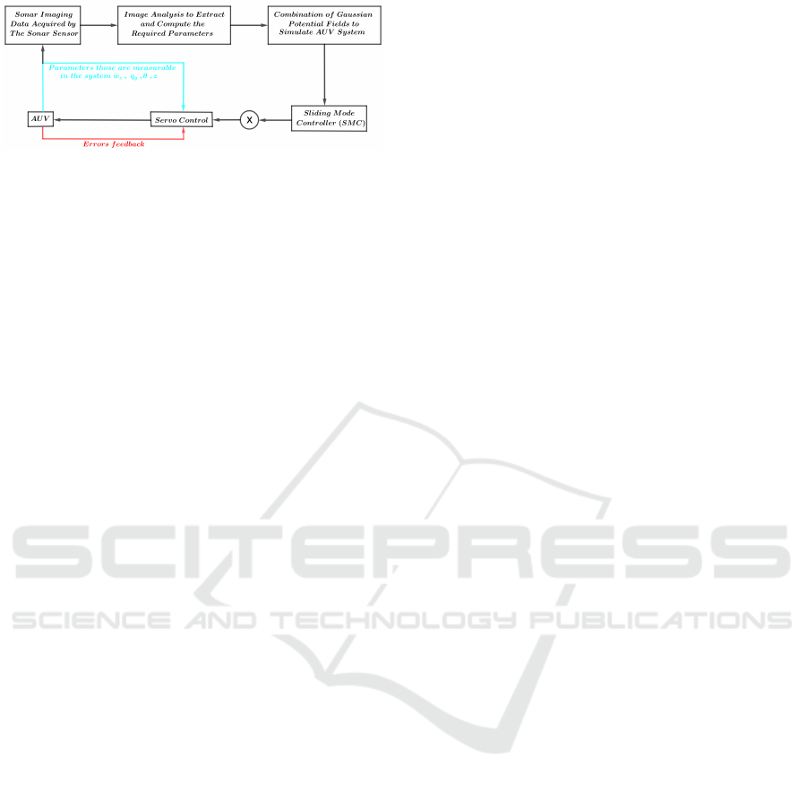
Figure 5: Schematic of AUV’s sliding mode controller.
during high-frequency switching scenarios. An AUV
experiment, featuring a simulated MRU and imag-
ing sonar, collected data to monitor the AUV’s depth
within a few meters. Employing a Gaussian poten-
tial function and an SMC controller with parameters
from processed sonar data, the AUV adjusted its tra-
jectory to avoid collisions by adapting its path based
on obstacle locations in sonar images (Figure 5). The
SMC controller offers advantages in underwater set-
tings, handling nonlinear behaviors and simplifying
system modeling, but challenges such as noise, sen-
sor malfunctions, and external disturbances need at-
tention. The AUV experiment demonstrated stability,
maintaining cruising height and avoiding collisions
using sonar images. Additional research is required
to assess SMC performance underwater, accounting
for noise and sensor failures.
5 SIMULATION RESULTS AND
DISCUSSION
5.1 Computational Domains for Pitch
Case Using CFD Interface
Using computational domains is essential in AUV
pitch analysis with CFD. A second domain simulates
different angles for diving and rising (Fig. 6). This
rectangular, parallelepiped-shaped domain extends by
1L before the bow and 2 L after the stern, with width
1 L and height 1.33 L, providing enough space for ma-
neuvering. CFD helps analyze fluid flow around the
AUV, crucial in underwater vehicle design and con-
trol.
5.2 Experimental Validation of SMC
Control for AUV
This study presents an AUV obstacle avoidance tech-
nique involving pitch and depth control. Front sonar
detects obstacles such as coral reefs or sea barriers
to prevent path obstruction. The AUV adjusts pitch
angle and depth for obstacle navigation. The sliding
mode controller computes an alternate path, pitching
up to the barrier’s height while maintaining distance.
Upon clearing the obstacle’s top, the AUV returns to
its original course by pitching down on the downward
slope. The sonar triggers the algorithm and supplies
obstruction size and range information. MATLAB
simulations utilized a developed sonar model to gen-
erate 2D images. Three seafloor types were explored
to address diverse mission scenarios.
The method simulates AUV navigation with
sonar-guided control, adjusting pitch and depth us-
ing a 2D domain. Different seafloor profiles are
compared. Sonar and MRU collaboratively enable
the AUV to autonomously navigate, avoiding ob-
stacles and maintaining course.Figure compares pro-
posed marine environment simulations with different
seafloor profiles. The AUV employs sonar beams,
generating images (Figures 9, 11, and 13) for obsta-
cle detection. The MRU and sonar jointly provide
a comprehensive view of the AUV’s surroundings,
enabling autonomous navigation, obstacle avoidance,
and course maintenance.
The method initially employs potential field-based
pitch and depth control for obstacle avoidance. How-
ever, Figure 8 reveals oscillatory response issues, ne-
cessitating AUV repositioning. Introducing sliding
mode control enhances efficiency and stability in ob-
stacle avoidance. SMC adjusts pitch and depth upon
obstacle detection, enabling safe navigation and im-
proved overall motion control for the AUV. By em-
ploying SMC, the AUV achieves precise and stable
trajectory, unaffected by external factors like ocean
currents or waves. As shown in Figure 9, the AUV
maintains a safe 90 m distance from a 4 m high ob-
stacle, effectively clearing it. Upon reaching the ob-
stacle’s top, pitch adjustment returns the AUV to its
original altitude. This method presents a promising
solution for AUV obstacle avoidance, enhancing nav-
igation in intricate and changing underwater environ-
ments.
The AUV effectively avoids collision, ascending
the barrier at approximately 33 m from the global
origin, despite a slight delay in the obstacle avoid-
ance SMC controller’s depth adjustments. Crucial ob-
stacle location and distance information is obtained
from front sonar images (Figure 10), assisting the
AUV’s trajectory adaptation. While response delay
is noted, successful collision avoidance demonstrates
a promising step towards improved and reliable AUV
obstacle avoidance methods.
Figure 11 accurately portrays obstacle height and
distance. The AUV’s controller adjusts stern sur-
faces, pitching the vehicle upward upon encounter-
ing the obstacle. The Gaussian potential field guides
Smooth Sliding Mode Control Based Technique of an Autonomous Underwater Vehicle Based Localization Using Obstacle Avoidance
Strategy
535

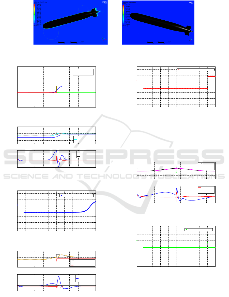
(a) (b)
Figure 6: Computational domain for pitch case: (a) Diving case, (b) Rising case.
0 20 40 60 80 100 120 140 160 180
−25
−20
−15
−10
−5
0
X (m)
Z−depth (m)
Seafloor wall
Gentle rise seafloor
Steep drop−off seafloor
Figure 7: Comparison of marine environment models.
0 20 40 60 80 100 120 140 160 180
−20
−10
0
X (m)
Z−depth (m)
0 20 40 60 80 100 120 140 160 180
−20
0
20
X (m)
Angle (°)
Depth control
Desired depth
Gentle rise seafloor
Steering angle
Pitch
True value
Figure 8: Analysis of AUV navigation dynamics along gen-
tle seafloor rise.
0 10 20 30 40 50 60 70 80 90 100
−8
−6
−4
−2
0
2
4
X
s
(m)
Y
s
(m)
Sonar gentle rise seafloor images
Figure 9: Observe sonar images of gentle seafloor rise.
0 20 40 60 80 100 120 140 160 180
−20
−10
0
X (m)
Z−depth (m)
0 20 40 60 80 100 120 140 160 180
−20
0
20
40
X (m)
Angle (°)
Depth control
Desired depth
Steep drop−off seafloor
Steering angle
Pitch
True value
Figure 10: Analyzing the dynamics of AUV navigation on
steep seafloor drop-off.
0 10 20 30 40 50 60 70 80 90 100
−8
−6
−4
−2
0
2
4
X
s
(m)
Y
s
(m)
Sonar steep drop−off seafloor images
Figure 11: Observe seafloor sonar images with steep drop-
off.
the AUV to a level altitude and its original trajectory.
This field’s attractive and repulsive forces effectively
steer the AUV to avoid obstacles, altering its path.
Real-time data from sonar sensors is essential for pre-
cise obstacle navigation in the environment.
0 20 40 60 80 100 120 140 160 180
−20
−10
0
X (m)
Z−depth (m)
0 20 40 60 80 100 120 140 160 180
−10
0
10
X (m)
Angle (°)
Depth control
Desired depth
Seafloor wall
Steering angle
Pitch
True value
Figure 12: Analysis of AUV navigation dynamics along
seafloor wall.
0 10 20 30 40 50 60 70 80 90 100
−8
−6
−4
−2
0
2
4
X
s
(m)
Y
s
(m)
Sonar seafloor wall images
Figure 13: Observe sonar images of the seafloor wall.
The combination of the Gaussian potential field
and sonar sensors effectively enables AUV obstacle
avoidance in both simulations and real-world scenar-
ios. This strategy ensures reliable navigation in intri-
cate underwater environments, as evidenced in Figure
ICINCO 2023 - 20th International Conference on Informatics in Control, Automation and Robotics
536

12. The SMC controller employs an internal Gaussian
potential field, facilitating the AUV’s maneuverability
around significant obstacles. By adjusting stern con-
trol surfaces, the controller induces controlled pitch-
ing within ±8
◦
range. The AUV follows the potential
field’s guidance until it successfully clears the obsta-
cle.
Figure 13 illustrates a trajectory that, though im-
practical due to the AUV’s limited maneuverabil-
ity and response time, emphasizes the potential field
method’s effectiveness in obstacle avoidance. The
method rapidly generates energy-based fields for real-
time obstacle avoidance, complemented by processed
front sonar images. Nonetheless, limitations exist,
such as addressing local minima, concave obstacles,
and AUV oscillations in confined spaces. Simulations
validate its proficiency in navigating structured envi-
ronments like seafloor walls.
6 CONCLUSIONS
This article delves into the obstacle avoidance abili-
ties of autonomous underwater vehicles through front
sonar sensors in the vertical plane. The research pro-
poses a sliding mode controller coupled with imaging
sonar to establish Gaussian potential fields, demon-
strating efficient obstacle avoidance. While the study
showcases successful outcomes, validation through
real sonar data across varied marine environments is
essential. The article suggests the utilization of mul-
tiple sonar sensors for a comprehensive 3D field of
view, aiming to eliminate blind spots.
Future AUV control research should prioritize im-
proving model accuracy and reliability. Enhance-
ments can involve extending the model to cover ad-
ditional motion planes and fine-tuning existing con-
trol systems. Integrating data from multiple sensors
can mitigate real-time state estimation uncertainties.
Waypoint navigation remains vital for autonomous
AUV control, with sliding mode controllers offering
stabilizing capabilities for roll, pitch, altitude, and ve-
locity tracking while managing estimated errors.
REFERENCES
Belker, T. and Schulz, D. (2002). Local action planning
for mobile robot collision avoidance. In Intelligent
Robots and System, IEEE/RSJ International Confer-
ence, pages 601–606.
Blidberg, D. (2003). The development of autonomous
underwater vehicles (auv). In A Brief Summary,
Autonomous Undersea Systems Institute, Lee New
Hampshire, USA.
Breivik, M. and Fossen, T. (2000). Guidance laws for au-
tonomous underwater vehicles. In Norwegian Univer-
sity of Science and Technology, Norway.
Coleman, J. (2003). Undersea drones pull duty in iraq hunt-
ing mines. In Cape Code Times.
Demim, F., Benmansour, S., Nemra, A., Rouigueb, A.,
Hamerlain, M., and Bazoula, A. (2022a). Simultane-
ous localization and mapping for autonomous under-
water vehicle using a combined smooth variable struc-
ture filter and extended kalman filter.
Demim, F. and et al., A. N. (2019). NH-∞-SLAM algorithm
for autonomous underwater vehicle.
Demim, F., Nemra, A., Abdelkadri, H., Louadj, K., Hamer-
lain, M., and Bazoula, A. (2018). Slam problem for
autonomous underwater vehicle using svsf filter. In
Proceeding of 25th IEEE International Conference
on Systems, Signals and Image Processing, Maribor,
Slovenia, pages 1–5.
Demim, F., Rouigueb, A., Nemra, A., Bouguessa, R., and
Chahmi, A. (2022b). A new filtering strategy for target
tracking application using the second form of smooth
variable structure filter. In Proceedings of the Institu-
tion of Mechanical Engineers, Part I: Journal of Sys-
tems and Control Engineering.
Desa, E., Madhan, R., and Maurya, P. (2001). Potential
of autonomous underwater vehicles as new genera-
tion ocean data platforms. In National Institute of
Oceanography, Dona Paula, India.
Healey, A. (2001). Dynamics and control of mobile robotic
vehicles. In Class Notes, Naval Postgraduate School,
Monterey, California, Winter.
Healey, A. and Kim, J. (2000). Control and random search-
ing with multiple robots. Proceedings IEEE CDC
Conference, Sydney Australia.
Issac, M., Adams, S., He, M., Neil, W., Christopher, D.,
and Bachmayer, R. (1979). Manoeuvring experiments
using the mun explorer auv. In In proceeding.
Khatib, O. (1986). Real-time obstacle avoidance for manip-
ulators and mobile robots.
Li, X. and Xiao, J. (2005). Robot formation control in
leader-follower motion using direct lyapunov method.
Prestero, T. (2009). Verification of a six-degree of free-
dom simulation model of remus autonomous under-
water vehicle. In MIT and WHOI.
Smooth Sliding Mode Control Based Technique of an Autonomous Underwater Vehicle Based Localization Using Obstacle Avoidance
Strategy
537