A Proactive Approach for the Sustainable Management of Water

Distribution Systems

Sarah Di Grande

, Mariaelena Berlotti

, Salvatore Cavalieri

and Roberto Gueli

Department of Electrical Electronic and Computer Engineering, University of Catania, Viale A. Doria n.6, Catania, Italy

EHT, Viale Africa n.31, Catania, Italy

Keywords: Water Distribution System, Water 4.0, Water Demand Forecasting, Energy Consumption Forecasting,

Machine Learning.

Abstract: Today, water distribution systems need to supply water to consumers in a sustainable way. This is connected

to the concept of Watergy, which means the satisfaction of user demand with the least possible use of water

and energy resources. Thanks to modern technologies, the forecasting of water and energy demand can help

achieve this goal. In particular, water demand forecasting allows water distribution companies to know in

advance how water resources will be allocated, it can help identify any anomalies in water consumption, and

it is essential for pumps scheduling. On the other hand, energy consumption forecasting has other important

roles, such as energy optimization, identification of anomalous consumption, and planning of energy load.

The present paper aims to develop short-term water demand and energy forecasting models through

innovative machine learning-based methodologies for the water distribution sector: global forecasting models,

the N-Beats machine learning algorithm, and transfer learning approaches. These tools demonstrated very

good performances in the creation of the models previously mentioned.

1 INTRODUCTION

Today water distribution systems (WDSs) are

responsible for water delivery with the required

quality, pressure, and quantity, but with the lowest

possible water and energy waste (Adedeji et al.,

2022), (Mesalie et al., 2021). This goal is linked to the

concept of Watergy efficiency, which means the

satisfaction of user demand with the least possible use

of water and energy resources (Bolognesi et al.,

2014).

Water scarcity poses a great threat to humans. It is

predicted that by 2025, 1.8 billion people may face

severe water shortages, and about two-thirds of the

world's population could be experiencing water stress

(Hans et al., 2014). This scenario of decreasing water

availability is the result of the amplification of

various factors, such as climate change, population

growth, increased urbanization rates, and industrial

development (Patil et al., 2022), (Leitão et al., 2019),

https://orcid.org/0009-0008-8895-2175

https://orcid.org/0009-0007-6564-704X

https://orcid.org/0000-0001-9077-3688

https://orcid.org/0000-0002-8014-0243

(de Souza Groppo et al., 2019), (Esen et al., 2020).

These phenomena have caused a significant increase

in water consumption reducing the available water

resources (Hussain et al., 2022), (Stańczyk et al.,

2022). Indeed, the increase in water consumption is

not accompanied by an increase in water resources.

Water demand forecasting can help in identifying

wasteful behavior or leakages in the system, which

lead not only to higher water consumptions but also

to higher energy consumption (Kofinas et al., 2016).

Furthermore, water demand forecasting prevents

energy waste through the possibility of pumps

scheduling, as it will be pointed out in the next

section.

Indeed, concerning energy consumption, a water

distribution system incurs high energy costs in all of

its operations (water extraction, treatment, and

distribution), but pumping systems are the biggest

cause of consumption (Sarmas et al., 2022). Luckily,

the optimal management of pumps’ operations, called

Di Grande, S., Berlotti, M., Cavalieri, S. and Gueli, R.

A Proactive Approach for the Sustainable Management of Water Distribution Systems.

DOI: 10.5220/0012121200003541

In Proceedings of the 12th International Conference on Data Science, Technology and Applications (DATA 2023), pages 115-125

ISBN: 978-989-758-664-4; ISSN: 2184-285X

 2023 by SCITEPRESS – Science and Technology Publications, Lda. Under CC license (CC BY-NC-ND 4.0)

115

pump scheduling can be a source of savings (Gan et

al., 2022). This concept would be better explained if

the Figure 1 has been considered.

Figure 1 is a simplified representation of how the

water is distributed to final users in a water

distribution network. In this network, each zone is

served by a pump system composed of 3

collaborating pumps (parallel pumps) that distribute

water collected in a reservoir. After each pump

system, there is a single pipe in which the water flows

to a network zone. Parallel pump systems give space

for energy savings opportunities because it can be

decided when to turn on/off pumps based on the water

demand and energy consumption (Gan et al., 2022).

In other words, not all pumps need to operate always

simultaneously, for example during the night when

the water demand is usually lower concerning

working hours.

Figure 1: A simple representation of a WDS.

In this context, forecasting the aggregated water

demand of each network zone plays a very important

role to schedule pumps’ operations. Accurate

forecasting helps in deciding how many and which

pumps to turn on at a given moment of the day based

on water demand. Furthermore, forecasting the

energy consumption of pump systems can also be

useful for different purposes: energy optimization,

identification of anomalous consumption, and

planning of energy load (Yi et al., 2022), (Alhendi et

al., 2022). In particular, the planning of the energy

load to be supported is fundamental to predicting the

necessary costs to be incurred and also if the system

will be able to cope with the required power.

In conclusion, today Watergy efficiency is the

main goal that water distribution companies want to

achieve and the digitalization that has pervaded the

management of water resources permits them to get

as close as possible to this goal. Indeed, the

sustainability of the water supply system would not

be possible without the industrial revolution of the

water sector, called Water 4.0 (Adedeji et al., 2022).

Automation, increased integration of sensors, Internet

of Things, big data analysis, and artificial intelligence

are some of the features of Water 4.0. In particular,

the most famous applications of artificial intelligence

in the management of water supply systems are

anomaly detection and water demand forecasting

(Adedeji et al., 2022). The present paper is focused

on the latter, together with the pumps’ energy

consumption forecasting. In particular, it is

implemented a 24-h horizon forecasting with a

timestep of 1 hour.

The proposal presented in the paper has been

developed inside a research project funded by “Italian

Ministry of Enterprises and Made in Italy”

(https://www.mimit.gov.it/en/); details about the

research project are given in the Acknowledgment

section. One of the partners of the project, EHT, is an

enterprise involved in the digital transformation of

water distribution systems. The goals of the research

here presented were specified by this enterprise

together with sponsors of the project, fully involved

in the same business area. Moreover, the enterprises

involved in the project evaluated the results achieved

in order to understand to what extent these results

could be valuable in practical terms; the evaluation of

these results was successful as the impact of the

proposal on the real management of water distribution

systems was considered important.

The paper is organized as it follows. In Section 2

the authors introduce related studies about machine

learning (ML) models used for water demand

forecasting and pumps energy forecasting. In Section

3 the authors describe the proposed approach to solve

the previously cited forecasting problems, explaining

how the dataset was simulated, the preprocessing

steps were done before the machine learning

algorithm, the proposed forecasting models, and

finally, the performance metrics used to evaluate

models. In Section 4 and Section 5 the obtained

results and conclusions with future works,

respectively, are reported.

2 RELATED WORKS

Water demand forecasting was addressed with

different machine learning forecasting models in the

literature. In (Niknam et al., 2022) and (de Souza

Groppo et al., 2019), a detailed review of the methods

employed, and important future challenges are given.

In particular, the three most used methods are in

order: traditional time series (e.g., autoregressive

integrated moving averages, exponential smoothing),

different types of artificial neural networks (e.g., long

DATA 2023 - 12th International Conference on Data Science, Technology and Applications

116

short-term memory, radial basis function ANN, gated

recurrent units), support vector machines.

Time series models are not able to reach high

accuracy forecasts as machine learning models,

because they are not able to learn complex, non-linear

patterns in demand forecasting. Despite this, they are

among the most used models due to their ease of use

and interpretation (Niknam et al., 2022). Among the

most recent papers, AutoRegressive Integrated

Moving Averages (ARIMA) and Exponential

Smoothing (ES) are the most used time series models.

In (Ebrahim Banihabib et al., 2019), two forecasting

methods for daily urban water consumption

forecasting are used; one of them is ARIMA. In

(Karamaziotis et al., 2020) different methods, among

which ARIMA and ES, are used to realize a mid-term

forecast. In (Ristow et al., 2021) the ARIMA and ES

methods are used to forecast monthly urban water

demand.

Regarding ANN, in (Salloom et al., 2021) an

hourly water demand forecasting with the Gated

Recurrent Unit (GRU) method is presented. In (Hu et

al., 2021), the GRU method is also used, but with the

aim to make an hourly water demand forecasting,

demonstrating the superiority of this method

compared to Support Vector Machines (SVM).

About the SVM method, in (Shabani et al., 2017),

it is used with a polynomial kernel function to predict

monthly water demand. In the paper (Candelieri et al.,

2019), the authors used the SVR with a parallel global

optimization tuning of hyperparameters, which

allowed them to increase the accuracy of the short-

term forecast.

The pumps’ energy consumption forecasting of a

water distribution system is instead a less explored

area of study. In (Yi et al., 2022), the authors used

four algorithms (multiple linear regression, random

forest, deep neural network, and support vector

regression) to forecast the energy consumption of an

entire water system and the three subsystems of

conveyance, treatment, and distribution. They

pointed out the lack of similar papers.

Partly according to the research carried out, and

partly also according to what was affirmed by

(Niknam et al., 2022), there are some quite

unexplored topics in literature.

In water distribution systems usually, water

demand time series are forecasted individually,

meaning that one model for each time series is

developed. Instead, global models could allow the

creation of a single model for all the time series

(Montero-Manso et al., 2021). This is essential

considering that, over the years, thanks to the

technologies available, the number of available series

will always increase, and new tools are needed to

manage it.

Furthermore, global models, learning from

multiple time series simultaneously, allow the use of

transfer learning approaches (Bandara et al., 2021). If

the model is trained on fairly heterogeneous series,

transfer learning should allow forecasting on series

never seen before.

Finally, to the best of the authors' knowledge,

among all the algorithms used, there is one that has

never been used in water demand and pumps’ energy

consumption forecasting of an entire water

distribution system: N-Beats (Oreshkin et al., 2020).

This is an algorithm developed specifically for time

series.

In summary, this paper aims to fill the gaps in the

literature by developing short-term water demand and

pumps’ energy consumption forecasting models

through global models using the N-Beats algorithm

and transfer learning approach.

3 DESCRIPTION OF THE

APPROACH

In this section, the authors describe the tools used for

data simulation, the dataset preprocessing phases, the

proposed forecasting method, and the performance

metrics for the models' evaluation.

3.1 Data Simulation

Data plays a strategic role in a machine learning

approach, as known. Considering the problem

presented in this paper, information about the WDS

like pipes flowrate and pumps’ energy consumption,

is strongly required. Data for water distribution

systems are often not available or of poor quality

(Maira et al., 2014). As the main aim of the paper was

the feasibility study of the proposed approach, data

needed to run the machine learning-based solution

was synthetically generated.

Data were simulated through Water Network Tool

for Resilience (WNTR), a Python package based

upon EPANET software, designed for the simulation

of water distribution networks (WDNs), version 0.5.0

(Klise et al., 2020). The WNTR simulator takes as

input an .inp file containing the network

characteristics (e.g., pipes, pumps, valves, junctions,

tanks, reservoirs, water demand patterns, pumps

curves) and it returns different time series with the

simulation results (e.g., pipes flowrate, nodes

pressure, pumps’ energy consumption).

A Proactive Approach for the Sustainable Management of Water Distribution Systems

117

The network used for the simulation is a

simplified version of the WDN of the city of Milano

(Italy); it is made up of 12,354 nodes, 17,548 links,

128 patterns, and 95 pump curves (one for each

pump). At each node representing a user, a water

demand pattern has been assigned. The demand

pattern was extrapolated from water consumption

data collected every minute on particular dates. More

in-depth, these consumption data were aggregated in

a dataset, where each column represented a specific

zone, and each row was the water consumption of a

particular minute of the day. In order to extract

coefficients of the general demand pattern, a column

with the total consumption per minute was added.

Finally, the column with the coefficients per minute

was obtained by dividing each observation of the total

consumption column by the average value of this

column. Then, the pattern was aggregated with the

mean operator to obtain 1-hour interval observations,

useful for the subsequent step of the hourly

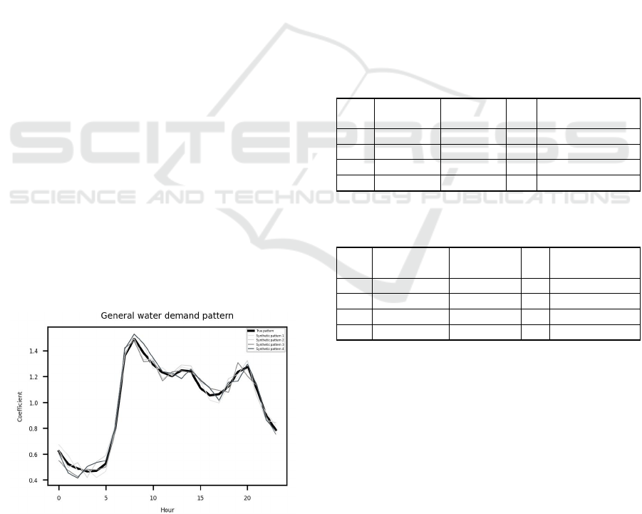
forecasting. True patterns of 24 hours are represented

by a black line in Figure 2.

From this real demand pattern, other 4 patterns

were obtained adding for each value of the true one a

random noise. In order to create a similar but different

pattern, at each value of the true pattern was added a

quantity that randomly increased or decreased the

original value. To calculate this quantity, first of all,

a random noise between -1.5 and 1.5 was generated

by multiplying a random value between 0 and 1 by 3

and subtracting 1.5. Then, this value was multiplied

by 0.05 to obtain a relative number between the 5%

of -1.5 and 1.5. For each value of the real pattern, this

process was repeated 4 times to obtain other 4 similar

patterns. Synthetic patterns of 24 hours are

represented in Figure 2 and compared with the true

values.

Figure 2: True water demand pattern and synthetic ones.

Even if this is the general water demand pattern,

in the network.inp file each node demanding water

has a specific base demand. This different base

demand for each node makes the demand pattern of

each node in the network unique.

Furthermore, the pump's speed was set constant

because WNTR at the moment doesn’t support

variable speed pumps.

The water distribution was simulated using this

network to obtain 5 days of hourly time series (120

observations). The simulation was a demand-driven

simulation, meaning that the pressure in the system

depends on the node demands, and that node demands

are always satisfied (Klise et al., 2020). The time

series collected to proceed with the analysis are:

flowrates series for each pipe (120 rows, 17548

columns), and energy consumption of each pump

(120 rows, 95 columns).

Table 1 and Table 2 provide an example of

flowrates and energy consumptions datasets,

respectively, where f indicates the flowrate and e is

the energy, while the index of the rows represents the

hours (120 of total hours because there are 5-day

hourly data).

Table 1: Simulated flowrates time series example.

Flow

ipe i

Flow

ipe i

… Flow

ipe i

17548

1,1

1,2

… f

1,17548

2,1

2,2

… f

2,17548

…… …… …

120 f

120,1

120,2

… f

120,17548

Table 2: Simulated energy consumptions time series

example.

Energy

id 1

Energy

id 2

… Energy

1,1

1,2

… e

1,95

2,1

2,2

… e

2,95

…… …… …

120 e

120,1

120,2

… e

120,95

3.2 Feature Selection

A feature selection procedure was done for both

flowrates dataset and pumps’ energy consumption

dataset to obtain the best input setting for the machine

learning algorithms.

As represented by Figure 1, after each group of

pumps there is a pipe from which water flows to a

zone based on the zone's aggregate water demand.

After this pipe, there would be many other pipes that

allow water to reach all the end users. Since the

authors were interested only in the aggregated

demand of a network area, for each served zone, the

pipe represented in Figure 1 was selected through its

DATA 2023 - 12th International Conference on Data Science, Technology and Applications

118

id, and the flowrates dataset was reduced from 17,548

to 27 columns (one pipe for each network zone).

Among the 27 time series, 7 of them showed an

almost constant pattern, and consequently, they were

excluded from the analysis. Therefore, a further

reduction was implemented from 27 to 20 columns

because the pipes of areas having an almost constant

simulated daily pattern were excluded.

The names of the selected zones of the Milano

network are: Anfossi, Armi, Assiano, Baggio,

Cantore, Chiusabella, Cimabue, Comasina,

Crescenzago, Feltre, Gorla, Italia, Lambro, Novara,

Padova, S. Siro, Salemi, Suzzani nord, Suzzani sud,

Vialba.

The final dataset was composed of 20 time series,

each one representing the 5-day aggregated water

demand of a network zone with an hourly interval.

The pumps’ energy consumption dataset needed a

first reduction of features to contain only the pumps’

energy consumption of the previously selected

network’s zones (from 95 to 72 pumps). Thus, a file

associating each pump with its area was consulted to

make the above selection. In each area, the pumps

collaborate for the delivery of water to the specific

zone. The number of collaborating pumps for each

area ranges from a minimum of 2 to a maximum of 5.

Furthermore, the consumption of pumps in the same

zone was aggregated with the sum operator to prepare

the dataset for the pumps’ energy consumption

forecasting of a network zone.

The final dataset was composed of 20 time series,

each one representing the 5-day aggregated pumps’

energy consumption of a network zone with an hourly

interval.

3.3 Model Definition

The aim of the paper is to develop machine learning

(ML) models for the aggregated water demand and

pumps’ energy consumption forecasting of 20

different water distribution network zones.

Each time series was normalized with the Min-

Max scaling so that the range of each variable

becomes 0-1. More specifically, given max the

maximum value of a variable, and min its minimum

value, each observation x is transformed according to

this formula:

𝑥𝑚𝑖𝑛

𝑚𝑎𝑥



𝑚𝑖𝑛

(1)

Then, to prepare the datasets for the machine

learning algorithms, each time series was divided into

a training set (first 4 days, 96 hours of observations)

and a test set (last day, 24 hours of observations).

The proposed forecasting approach is shown

below in Figure 3 and Figure 4.

All machine learning models were performed

through Darts (version 0.23.1), a Python machine

learning library specific for time series analysis, in

particular for time series forecasting (Herzen et al.,

2022). The powerful feature of Darts is to provide

modern machine learning functionalities with a user-

friendly and easy-to-use API design (Herzen et al.,

2022). Furthermore, all deep learning forecasting

models implemented in Darts are global forecasting

models. A global forecasting model has great

potential because it can be trained with multiple time

series and it can make forecasting not only for these

time series but also for unseen series (transfer

learning approach).

Other important information about the training of

global forecasting models will be provided in the next

paragraph, together with detailed information on the

architecture of the used model.

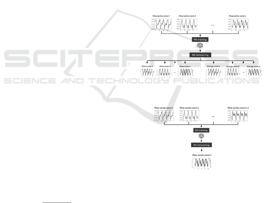
Figure 3: Water demand and pumps’ energy consumption

forecasting through a unique ML model trained with

flowrates series.

Figure 4: Water demand forecasting for one zone through a

ML model trained with all the flowrates series excluding

the forecasted one.

As depicted by Figure 3 and Figure 4, the water

demand forecasting of each flowrate time series was

addressed with two different methodologies.

The first consists in the creation of a global

forecasting model taking as input all the flowrates

series training sets, and giving 24 hours of forecast

A Proactive Approach for the Sustainable Management of Water Distribution Systems

119

for all of these series (Figure 3). The Darts model

used for forecasting is the N-Beats model. The default

hyperparameters were maintained except for two of

them: the input_chunk_length and the

output_chunk_length. The former specifies the length

of the time series portion taken in input by the internal

neural network and was set to 72, meaning that the

neural network looks 72 hours in the past. The latter

represents the length of the forecast of the model and

was set to 24, meaning that the neural network

produces 24 points of forecast.

The second method consists in the creation of a

global forecasting model for each flowrate series

taking as input all the flowrates series training sets

except for this one, and giving 24 hours of forecast

for this series. This approach exploits the knowledge

gained with the training of some series to forecast

unseen series (transfer learning). Figure 4 represents

an example of this method applied for the forecasting

of a single flowrate series.

The latter method was applied also for the

construction of the pumps’ energy consumption

forecasting model. The energy consumption of pumps

strictly depends on the flowrate pattern. The WNTR

simulator calculates it considering the pump flowrate,

the node head, and the global efficiency of the pump

(set to 75%). Therefore, each pump’s energy

consumption time series has almost the same pattern

as the flowrate time series in the same network zone.

Instead of creating an additional model, the first

global model trained with all the flowrates time series

was tested for the energy consumption forecasting of

each zone (see Figure 3).

3.4 N-Beats Global Forecasting Model

This section provides insights into the used model (N-

Beats) and how the training of global models works

on the Darts library.

Recently, the authors of (Oreshkin et al., 2020)

proposed a neural network architecture designed for

time series forecasting called N-Beats (Neural basis

expansion analysis for interpretable time series

forecasting). In the following, the architecture of the

model will be described, as shown in Figure 5; more

details may be achieved by (Oreshkin et al., 2020).

Given a forecast horizon (or forecast period) of

length H and an observed series history (or lookback

period) of length T (where T = n × H), the model takes

as input the lookback period to learn the behavior of

the time series, and it predicts the behavior of the

same time series in the forecast period (upper part of

Figure 5). There are different stacks (right part of

Figure 5), and at the end, the output of each stack is

combined to obtain a global forecasting output. In

each stack, there are multiple blocks (middle part of

Figure 5), and each block has a fully connected stack

with 4 layers that do both forecasting and backcasting

(left part of Figure 5). The difference between

forecasting and backcasting is the direction of

predictions: the former predicts future values by

looking back at historical data, and the latter

extrapolate past values from future data (forecasting

backward in time). Furthermore, nonlinearities are

provided by the ReLU activation function. Activation

functions have an important task because they

introduce non-linearities in the network. In other

words, learning complex pattern in the data, help in

the resolution of real-world problems. There are

different activation functions that can be used in the

network, but the ReLU (rectified linear unit) is the

most popular because it is simple and fast (Nair et al.,

2010).

Figure 5: N-Beats architecture.

This model has been used through the Darts

Python library. Darts library has implemented many

forecasting models, but only a subset of them can be

trained with multiple time series (among which N-

Beats). These models are called global forecasting

models. Time series can be divided into two classes:

target time series (series to be forecasted) and

covariate time series (series not to be forecasted but

to be taken into consideration to help target time

series forecasting). The present paper does not

consider the presence of covariates, therefore models

take in input only target series. This choice lies in the

fact that water demand history is the main factor

influencing future demand, therefore it is sufficient

for developing accurate models (Hu et al., 2021),

(Bakker et al., 2013).

When a model with multiple target time series

needs to be trained (as in our case), Darts creates a

dataset aggregating multiple input/output pairs from

the provided time series. The length of the input is

equal to the input_chunk_length hyperparameter,

DATA 2023 - 12th International Conference on Data Science, Technology and Applications

120

while the length of the output depends on the

output_chunk_length hyperparameter.

Figure 6 shows the training phase of a model with

two example series of different lengths and different

time stamps in input.

In this example, the input_chunk_length is equal

to 4, while the output_chunk_length is equal to 2. The

number of samples used for training is calculated by

subtracting from the time series length the sum of the

input_chunk_length and output_chunk_length, and

adding 1 to this result. Therefore, the first series has a

number of samples used for training equal to 9, while

the number of samples of the second series is 7. A

training epoch in multiple series models consists of

the complete pass over all the samples of all the

series. Finally, the most important things to point out

are that series do not need to have the same length,

the same time stamps, or the same frequency

(although this is not our case).

Figure 6: Training of global models in Darts library.

3.5 Performance Metrics

Different metrics were considered for the

performance evaluation of forecasting models: mean

absolute error (MAE), symmetric mean absolute

percentage error (SMAPE), mean squared error

(MSE), and root mean square error (RMSE).

MAE is a measure of error between predicted and

true values, and it is calculated as an arithmetic

average of the absolute errors (Hyndman et al., 2006).

SMAPE is a measure of accuracy based on

relative errors, therefore it is a percentage value

(Hyndman et al., 2006), (Bandara et al., 2021).

MSE is a measure indicating the average squared

difference between predicted values and actual values

(Hyndman et al., 2006).

RMSE is calculated as the square root of the mean

of the square of all the errors (Hyndman et al., 2006).

For all of these measures, the lower the values, the

better the model performance.

4 RESULTS

In this work, innovative machine-learning based

methodologies are proposed to develop short-term

water demand and energy forecasting models. This

important task was addressed with the use of global

forecasting models and transfer learning approaches.

First of all, four different global models were

tested to select the one that provided the most

accurate water demand forecasting. Among the

models available within the Darts python library, the

ones that were tested are: N-Beats, RNN, BlockRNN,

and Transformer.

Performance metrics are reported in Table 3.

Table 3: Performance metrics of N-Beats, RNN,

BlockRNN, and Transformer global models.

N-Beats RNN Block RNN Transf

MAE 0.031 0.188 0.23 0.16

SMAPE 21.322 52.15 56.174 45.762

MSE 0.003 0.06 0.075 0.043

RMSE 0.043 0.237 0.265 0.194

Among the models used, the N-Beats model

outperforms the others according to all metrics

considered, confirming its superiority in terms of

forecasting accuracy. The other algorithms obtained

very similar metrics’ results, and the following

ranking was obtained in decreasing order of

performance: N-Beats, Transformer, RNN,

BlockRNN. Taking as an example the SMAPE

metric, it can be seen that considering the N-Beats

model this metric is reduced by more than half

compared to all the other models. The

outperformance of this model may be attributed to its

ability to do both backcasting and forecasting, which

is a property that greatly differentiates it from the

other algorithms, as said before in Section 3.4 while

describing its architecture.

The performance metrics of the N-Beats global

forecasting model (Table 3, first column) have been

compared to the ones obtained from the creation of

single models trained with one series at a time; in this

case, the following values have been achieved:

MAE=0.030, SMAPE=21.839, MSE=0.003, RMSE=

0.043. As it can be easily pointed out, almost identical

results have been achieved. This situation may have

been arisen because a restricted amount of data was

used, but building a global forecasting model trained

with a lot of real data with a longer period of time may

benefit from learning from more patterns at the same

time. Indeed, related time series could improve the

overall predictions with respect to the result obtained

with a collection of local models (Hewamalage et al.,

2022). However, the time spent for training one

model with multiple time series was lower than the

total time needed to train a model for each series (36

seconds and 476 seconds respectively). This could be

justified considering that the model complexity of

A Proactive Approach for the Sustainable Management of Water Distribution Systems

121

local models grows proportionally to the number of

time series in the dataset, and it can be higher than the

constant complexity of the global model

(Hewamalage et al., 2022). As said in Section 1, in

the Water 4.0 era, water distribution systems are

characterized by increased integration of sensors,

Internet of Things, and big data. As a result, so much

more data can be collected, analyzed, and exploited

in the decision-making and planning phases.

However, having access to all this information also

means learning how to manage it properly. The

results obtained demonstrate that the use of global

models meets these needs, as forecasting can be

performed by training a single model on multiple

series with less time spent than creating multiple local

models.

Pumps energy consumption patterns strictly

depends on the water demand of the respective zone.

For this reason, the previously created model trained

with water demand time series has been used to reach

the goal of pumps’ energy consumption forecasting.

Performance metrics results demonstrate the

effectiveness of the approach (MAE: 0.032; SMAPE:

21.305; MSE: 0.003; RMSE: 0.043).

Finally, it has been explored the capacity of global

forecasting models to forecast previously unseen

series. For each flowrate time series, it has been

created a model trained with all the other series and

tested with this excluded one. Out of 20 forecasts, 18

of them produce very good results, demonstrating the

ability of the models to generalize well (MAE: 0.079;

SMAPE: 25.141; MSE: 0.012; RMSE: 0.1), while the

other two have been considered unacceptable

forecasting (MAE: 0.203; SMAPE: 97.746; MSE:

0.057; RMSE: 0.238). The worst performance of

transfer learning in this small group of time series

may be attributed to the fact that the patterns of these

time series are too different from the group of time

series on which the model is trained. Consequently,

the fact that these two series have a totally different

pattern from the others suggests that a global model

made up of as heterogeneous series as possible can

obtain better performances in the case of transfer

learning.

A few examples of comparisons between the

forecasting of global forecasting models and transfer

learning models are reported in Figure 7, Figure 8,

and Figure 9.

In conclusion, an essential step in the water and

energy forecasting approach is to compare the results

of this study with similar research in the past

literature. However, no comparative research was

found as the use of global models, the N-Beats

algorithm, and transfer learning techniques is a field

being explored for the first time in the water

distribution sector.

Figure 7: Water demand forecasting for the zone named

Cimabue with the global forecasting model and the pre-

trained model.

Figure 8: Water demand forecasting for the zone named

Comasina with the global forecasting model and the pre-

trained model.

DATA 2023 - 12th International Conference on Data Science, Technology and Applications

122

Figure 9: Water demand forecasting for the zone named

Feltre with the global forecasting model and the pre-trained

model.

5 CONCLUSIONS

In this study, the authors developed a short-term

water demand and pumps’ energy consumption

forecasting with simulated data from the Milano

water distribution network. In particular, hourly data

were used to make 24-h horizon forecasts.

To the best of the authors' knowledge, the

approaches proposed for forecasting differ from

previously published studies in different points.

First of all, both water and energy forecasts are

investigated together for the same water distribution

network.

Then, it is the first time that global models are

used in the water sector, and this has made it possible

to create fast a single and general model able to

generalize on unseen time series (transfer learning).

Finally, although N-Beats was never used before

in the water demand and pumps’ energy consumption

forecasting of an entire water distribution system, the

results achieved by the authors pointed out that it

offered the best performance; on account of these

results, it seems very suitable to be used in this field.

Future studies plan to test this methodology with

real data covering a longer period, to create more

complex models able to detect weekdays, weekends,

and yearly patterns, or trends if present. Furthermore,

also mid-term and long-term forecasts could be

developed.

ACKNOWLEDGEMENTS

The research results presented in this paper have been

achieved inside the Water 4.0 project, named

“Technologies for the convergence between industry

4.0 and the integrated water cycle”. This research

project is currently running and is funded by the

Ministry of Enterprises and Made in Italy

(https://www.mimit.gov.it/en/).

REFERENCES

Adedeji, K. B., Ponnle, A. A., Abu-Mahfouz, A. M.,

Kurien, A. M. (2022). Towards Digitalization of Water

Supply Systems for Sustainable Smart City

Development—Water 4.0. Applied Sciences, 12, 9174.

MDPI. https://doi.org/10.3390/app12189174

Alhendi, A. A., Al-Sumaiti, A. S., Elmay, F. K., Wescaot,

J., Kavousi-Fard, A., Heydarian-Forushani, E.,

Alhelou, H. H. (2022). Artificial intelligence for water–

energy nexus demand forecasting: a review.

International Journal of Low-Carbon Technologies, 17,

730–744. Oxford University Press. https://doi.org/10.

1093/ijlct/ctac043

Bakker, M., Vreeburg, J. H. G., van Schagen, K. M.,

Rietveld, L. C. (2013). A fully adaptive forecasting

model for short-term drinking water demand.

Environmental Modelling & Software, 48, 141-151.

ELSEVIER. https://doi.org/10.1016/j.envsoft.2013.06.

012

Bandara, K., Hewamalage, H., Liu, Y.-H., Kang, Y.,

Bergmeir, C. (2021). Improving the accuracy of global

forecasting models using time series data augmentation.

Pattern Recognition, 120, 108148. ELSEVIER.

https://doi.org/10.1016/j.patcog.2021.108148

Bolognesi, A., Bragalli, C., Lenzi, C., Artina, S. (2014).

Energy efficiency optimization in water distribution

systems. Procedia Engineering, 70, 181-190.

ELSEVIER. https://doi.org/10.1016/j.proeng.2014.02.

021

Candelieri, A., Giordani, I., Archetti, F., Barkalov, K.,

Meyerov, I., Polovinkin, A., Sysoyev, A., & Zolotykh,

N. (2019). Tuning hyperparameters of a SVM-based

water demand forecasting system through parallel

global optimization. Computers & Operations

Research, 106, 202-209. ELSEVIER. https://doi.

org/10.1016/j.cor.2018.01.013

de Souza Groppo, G., Costa, M. A., Libânio, M. (2019).

Predicting water demand: a review of the methods

employed and future possibilities. Water Supply, 19(8),

A Proactive Approach for the Sustainable Management of Water Distribution Systems

123

2179-2198. IWA PUBLISHING. https://doi.org/10.

2166/ws.2019.122

Ebrahim Banihabib, M., Mousavi-Mirkalaei, P. (2019).

Extended linear and non-linear auto-regressive models

for forecasting the urban water consumption of a fast-

growing city in an arid region. Sustainable Cities and

Society, 48, 101585. ELSEVIER. https://doi.org/10.

1016/j.scs.2019.101585

Esen, Ö., Yıldırım, D. Ç., Yıldırım, S. (2020). Threshold

effects of economic growth on water stress in the

Eurozone. Environmental Science and Pollution

Research, 27, 31427–31438. Springer. https://doi.org

/10.1007/s11356-020-09383-y

Gan, X., Pei, J., Pavesi, G., Yuan, S., Wang, W. (2022).

Application of intelligent methods in energy efficiency

enhancement of pump system: A review. Energy

Reports, 8, 11592–11606. ELSEVIER. https://doi.org/

10.1016/j.egyr.2022.09.016

Hans, A., Bharat, D. A. (2014). Water as a Resource:

Different Perspectives in Literature. International

Journal of Engineering Research, 3(10). IJERT. DOI:

10.17577/IJERTV3IS100054.

Herzen, J., Lässig, F., Piazzetta, S. G., Neuer, T., Tafti, L.,

Raille, G., Van Pottelbergh, T., Pasieka, M., Skrodzki,

A., Huguenin, N., Dumonal, M., Kościsz, J., Bader, D.,

Gusset, F., Benheddi, M., Williamson, C., Kosinski,

M., Petrik, M., Grosch, G. (2023). Darts: User-friendly

modern machine learning for time series. The Journal

of Machine Learning Research, 23, 1-6. arXiv.

https://doi.org/10.48550/arXiv.2110.03224

Hewamalage, H., Bergmeir, C., Bandara, K. (2022). Global

models for time series forecasting: A Simulation study.

Pattern Recognition, 124, 108441. ELSEVIER.

https://doi.org/10.1016/j.patcog.2021.108441

Hu, S., Gao, J., Zhong, D., Deng, L., Ou, C., Xin, P. (2021).

An Innovative Hourly Water Demand Forecasting

Preprocessing Framework with Local Outlier

Correction and Adaptive Decomposition Techniques.

Water, 13(5), 582. MDPI. https://doi.org/

10.3390/w13050582

Hussain, Z., Wang, Z., Wang, J., Yang, H., Arfan, M.,

Hassan, D., Wang, W., Azam, M. I., Faisal, M. (2022).

A comparative Appraisal of Classical and Holistic

Water Scarcity Indicators. Water Resources

Management, 36, 931-950. Springer. https://doi.org/

10.1007/s11269-022-03061-z

Hyndman, R. J., Koehler, A. B. (2006). Another look at

measures of forecast accuracy. International Journal of

Forecasting, 22(4), 679-688. ELSEVIER. https://doi.

org/10.1016/j.ijforecast.2006.03.001

Karamaziotis, P. I., Raptis, A., Nikolopoulos, K., Litsiou,

K., Assimakopoulos, V. (2020). An empirical

investigation of water consumption forecasting

methods. International Journal of Forecasting, 36(2),

588-606. ELSEVIER. https://doi.org/10.1016/j.

ijforecast.2019.07.009

Klise, K., Hart, D., Bynum, M., Hogge, J., Haxton, T.,

Murray, R., Burkhardt, J. (2020). Water Network Tool

for Resilience (WNTR). User Manual, Version 0.2.3.

EPA. https://doi.org/10.2172/1660790

Kofinas, D., Papageorgiou, E., Laspidou, C., Mellios, N.,

Kokkinos, K. (2016). Daily Multivariate Forecasting of

Water Demand in a Touristic Island with the Use of

Artificial Neural Network and Adaptive Neuro-Fuzzy

Inference System. 2016 International Workshop on

Cyber-Physical Systems for Smart Water Networks

(CySWater), Vienna, Austria. IEEE. https://doi.org/

10.1109/CySWater.2016.7469061

Leitão, J., Simões, N., Sá Marques, J. A., Gil, P., Ribeiro,

B., Cardoso, A. (2019). Detecting urban water

consumption patterns: a time-series clustering

approach. Water Supply, 19(8), 2323-2329. IWA

PUBLISHING. https://doi.org/10.2166/ws.2019.113

Maira, M., Raucha, W., Sitzenfreia, R. (2014). Improving

incomplete water distribution system data. 12th

International Conference on Computing and Control

for the Water Industry (CCWI2013), Procedia

Engineering 70 (2014) 1055 – 1062.

Mesalie, R. A., Aklog, D., Kifelew, M. S. (2021). Failure

assessment for drinking water distribution system in the

case of Bahir Dar institute of technology, Ethiopia.

Applied Water Science, 11, 138. Springer.

https://doi.org/10.1007/s13201-021-01465-7

Montero-Manso, P., Hyndman, R. J. (2021). Principles and

Algorithms for Forecasting Groups of Time Series:

Locality and Globality. International Journal of

Forecasting, 37, 1632-1653. arXiv. https://doi.org/10.

1016/j.ijforecast.2021.03.004

Nair, V., Hinton, G. E. (2010). Rectified Linear Units

Improve Restricted Boltzmann Machines. Proceedings

of the 27 th International Conference on Machine

Learning, Haifa, Israel, 2010. ACM.

Niknam, A., Zare, H. K., Hosseininasab, H., Mostafaeipour,

A., Herrera, M. (2022). A Critical Review of Short-

Term Water Demand Forecasting Tools—What

Method Should I Use? Sustainability, 14(9), 5412.

MDPI. https://doi.org/10.3390/su14095412

Oreshkin, B. N., Carpov, D., Chapados, N., Bengio, Y.

(2020). N-BEATS: Neural basis expansion analysis

for interpretable time series forecasting.

(arXiv:1905.10437). arXiv. https://doi.org/10.48550/

arXiv.1905.10437

Ristow, D. C. M., Henning, E., Kalbusch, A., Petersen, C.

E. (2021). Models for forecasting water demand using

time series analysis: A case study in Southern Brazil.

Journal of Water, Sanitation and Hygiene for

Development, 11(2), 231-240. IWA PUBLISHING.

https://doi.org/10.2166/washdev.2021.208

Salloom, T., Kaynak, O., He, W. (2021). A novel deep

neural network architecture for real-time water demand

forecasting. Journal of Hydrology, 599, 126353.

ELSEVIER. https://doi.org/10.1016/j.jhydrol.2021.

126353

Sarmas, E., Spiliotis, E., Marinakis, V., Tzanes, G.,

Kaldellis, J. K., Doukas, H. (2022). ML-based energy

management of water pumping systems for the

application of peak shaving in small-scale islands.

Sustainable Cities and Society, 82, 103873.

ELSEVIER. https://doi.org/10.1016/j.scs.2022.103873

DATA 2023 - 12th International Conference on Data Science, Technology and Applications

124

Shabani, S., Yousefi, P., Naser, G. (2017). Support Vector

Machines in Urban Water Demand Forecasting Using

Phase Space Reconstruction. Procedia Engineering,

186, 537–543. ELSEVIER.

https://doi.org/10.1016/j.proeng.2017.03.267

Stańczyk, J., Kajewska-Szkudlarek, J., Lipiński, P.,

Rychlikowski, P. (2022). Improving short-term water

demand forecasting using evolutionary algorithms.

Scientific Reports, 12, 13522. Nature publishing group.

https://doi.org/10.1038/s41598-022-17177-0

Yi, S., Kondolf, G. M., Sandoval-Solis, S., Dale, L. (2022).

Application of Machine Learning-based Energy Use

Forecasting for Inter-basin Water Transfer Project.

Water Resources Management, 36, 5675–5694.

Springer. https://doi.org/10.1007/s11269-022-03326-7.

A Proactive Approach for the Sustainable Management of Water Distribution Systems

125