Source-Code Embedding-Based Software Defect Prediction

Diana-Lucia Miholca

and Zsuzsanna Onet¸-Marian

Department of Computer Science, Babes¸-Bolyai University, No. 1, Mihail Kogalniceanu street, Cluj-Napoca, Romania

Keywords:

Software Defect Prediction, Doc2Vec, Graph2Vec, LSI, Hyperparameter Tuning, Deep Learning.

Abstract:

Software defect prediction is an essential software development activity, a highly researched topic and yet a

still difﬁcult problem. One of the difﬁculties is that the most prevalent software metrics are insufﬁciently rel-

evant for predicting defects. In this paper we are proposing the use of Graph2Vec embeddings unsupervisedly

learnt from the source code as basis for prediction of defects. The reliability of the Graph2Vec embeddings

is compared to that of the alternative embeddings based on Doc2Vec and LSI through a study performed on

16 versions of Calcite and using three classiﬁcation models: FastAI, as a deep learning model, Multilayer

Perceptron, as an untuned conventional model, and Random Forests with hyperparameter tuning, as a tuned

conventional model. The experimental results suggest a complementarity of the Graph2Vec, Doc2Vec and

LSI-based embeddings, their combination leading to the best performance for most software versions. When

comparing the three classiﬁers, the empirical results highlight the superiority of the tuned Random Forests

over FastAI and Multilayer Perceptron, which conﬁrms the power of hyperparameter optimization.

1 INTRODUCTION

Software defect prediction (SDP) is the task of iden-

tifying defective software components, so that testing

effort can be focused on them. Since the resources

for testing are always limited, having accurate SDP

models can lead to the best results with the available

resources. Given its importance, it is not surprising

that SDP is an actively researched topic.

In order to build a Machine Learning (ML) model

for SDP it is necessary to have a common represen-

tation (feature vector) for all the software entities.

The earliest and prevalent representation is based on

software metrics. Initially, the metrics considered

have been procedural code metrics exclusively, but

they have been replaced (or complemented) later by

object-oriented and code change metrics.

More recently, however, several approaches for

constructing software features by directly or indi-

rectly considering the source code, through the Ab-

stract Syntax Tree (AST), have been proposed.

In a recent study (Miholca et al., 2022), an exten-

sive series of traditional software metrics have been

compared to conceptual software features extracted

directly from the source code using Doc2Vec and

LSI. The study’s conclusion is that, on average, the

https://orcid.org/0000-0002-3832-7848

https://orcid.org/0000-0001-9006-0389

Doc2Vec and LSI-based software features outperform

the traditional ones in terms of their soundness in pre-

dicting defect-proneness. In extracting the Doc2Vec

and LSI-based features, the source code is seen as a

piece of text. So, its actual structure, which is cap-

tured by the AST, is not taken into consideration.

Consequently, in the current paper, we want to

build on the work of Miholca et al. (Miholca et al.,

2022), while also capitalizing on the structure under-

lying the source code. To this end, we are proposing

an additional representation unsupervisedly learnt

from the AST of the source code using Graph2Vec

(Narayanan et al., 2017). Graph2Vec is a neural

embedding framework which can learn a ﬁxed-length

feature vector (called embedding) for an entire

graph. The Graph2Vec-based embeddings will be

evaluated in terms of their discriminative power when

it comes to classifying software entities as defective

or non-defective. Having the intuition of a possible

complementarity between the Graph2Vec-based

embedding, that capitalizes on the software structure,

and the Doc2Vec and LSI-based embeddings, that

capitalize on the semantics of the source code (espe-

cially of the comments and identiﬁers), we will also

investigate if combining them leads to a superior SDP

performance. Accordingly, we deﬁne the following

research questions:

Miholca, D. and OneÅ

c-Marian, Z.

Source-Code Embedding-Based Software Defect Prediction.

DOI: 10.5220/0012129600003538

In Proceedings of the 18th International Conference on Software Technologies (ICSOFT 2023), pages 185-196

ISBN: 978-989-758-665-1; ISSN: 2184-2833

 2023 by SCITEPRESS – Science and Technology Publications, Lda. Under CC license (CC BY-NC-ND 4.0)

185

• RQ1. What is the relative relevance of the embed-

ding learnt using Graph2Vec for SDP?

• RQ2. Does the combination of the Graph2Vec,

Doc2Vec and LSI embeddings improve the per-

formance of SDP?

Miholca et al. (Miholca et al., 2022) have experimen-

tally compared multiple classiﬁers of which FastAI

proved to be the best performer, being followed by a

feed-forward artiﬁcial neural network that is, in fact,

a Multilayer Perceptron (MLP). Since we build on

their results and conclusions, we will also use FastAI,

which is a deep learning model. However, recently,

some studies (for example (Fu and Menzies, 2017)

and (Majumder et al., 2018)) have shown that there

are many tasks for which there is no need for deep

learning, which in general needs more training data

and takes a longer time to run, since the same perfor-

mance can be achieved with a simpler ML algorithm

if proper hyperparameter tuning is performed. While

these studies considered other tasks, not SDP, Tan-

tithamthavorn et al. in (Tantithamthavorn et al., 2019)

investigated the impact of automated parameter opti-

mization for SDP and concluded that for most classi-

ﬁcation techniques a non-negligible performance im-

provement can be achieved by hyperparameter opti-

mization. Starting from this conclusion, we have de-

cided to use the Random Forest (RF) classiﬁer with

optimized parameters as well. Consequently, we add

a third research question:

• RQ3. How does the SDP performance of FastAI

compare to the one of RF with optimized param-

eters for the considered representations?

The main original contributions brought by this pa-

per are as follows. To the best of our knowledge, the

Graph2Vec-based embedding learnt from the source

code AST has not yet been used as representation

in the SDP literature. This being the case, we are

proposing a new software representation for the ben-

eﬁt of SDP. Moreover, we are proposing combining

the Graph2Vec-based embedding with the Doc2Vec-

based and the LSI-based embeddings proposed in

(Miholca et al., 2022) to unite the power of structural

and conceptual information underlying the source

code and thus to boost the SDP performance. In ad-

dition to this contributions, in this paper we are also

assessing the potency of parameter optimization in the

context of SDP by comparing a tuned Random Forest

to the FastAI deep classiﬁer, while feeding them with

the proposed software embeddings.

The remainder of this paper is organized in the fol-

lowing manner. Section 2 shortly presents a selection

of existing SDP approaches that are relevant for the

current paper. Section 3 describes in detail the experi-

mental methodology. Section 4 presents the results of

the performed analysis and formulates the answers to

our research questions. Finally, in Section 5, the con-

clusions are drawn and some directions to continue

this work are outlined.

2 RELATED WORK

There is a huge amount of literature related to the

problem of SDP. Throughout the years, researchers

proposed many approaches using supervised and un-

supervised machine learning, deep learning, ensem-

ble approaches, etc. In the following we will focus

only on a selection of papers that are most related to

the main topic of our paper: different software repre-

sentations to be used in SDP.

Most existing studies use for experimental evalu-

ation the SDP data sets available in Promise Software

Engineering Repository (Sayyad and Menzies, 2015),

that is currently known as SeaCraft (Sea, 2017). Ac-

cordingly, many of the existing SDP approaches are

based on the Promise metrics, that are either static OO

metrics or traditional metrics associated with the qual-

ity of the procedural source code. Literature reviews

reveals that about 87% (Malhotra, 2015) of the case

studies used such procedural or object-oriented met-

rics while being focused on proposing accurate clas-

siﬁers.

However, relatively recent studies have opened up

a new, highly active, research direction in the ﬁeld

of SDP - the one of designing new relevant features

for enabling the discrimination between defective and

non-defective software entities. This research direc-

tion is motivated by the fact that the existing software

features are insufﬁcient or insufﬁciently relevant for

SDP, making it still a difﬁcult problem. In the fol-

lowing, we will focus on presenting state-of-the art

approaches that are the most related to our approach.

Many approaches proposing new features con-

sider the AST of the source code. One such approach

is presented by Wang et al. in (Wang et al., 2016)

and (Wang et al., 2020). They automatically learn

semantic features starting from the AST and using

Deep Belief Networks (DBNs). The resulted features

have been comparatively evaluated against traditional

metrics in terms of their relevance for SDP, on open

source projects from the Promise repository as case

studies. The evaluation results have conﬁrmed that

the proposed semantic features outperform traditional

SDP features.

Li et al (Li et al., 2017) have proposed a simi-

lar process, but using Convolutional Neural Networks

(CNNs) instead of DBNs, and combining the ex-

ICSOFT 2023 - 18th International Conference on Software Technologies

186

tracted features with some traditional ones. The com-

bined representation has been evaluated in terms of its

soundness for SDP by using the Logistic Regression

(LR) classiﬁer. The results of the experimental eval-

uation conﬁrmed that the AST-based features outper-

form traditional features, while combining the two of

them leads to even better performance.

Another study using AST-based features for SDP

is the one performed by Dam et al. (Dam et al.,

2018). They have introduced a tree-structured net-

work of Long-Short Term Memory (LSTM) units as a

SDP model starting from AST embeddings. Using the

same set of 10 case studies as Wang et al. (Wang et al.,

2016), they train two traditional classiﬁers: LR and

Random Forest on the features generated by LSTM.

Aladics et al. (Aladics et al., 2021) have pro-

posed an approach, where the AST of the source code

was parsed in a depth-ﬁrst order, and the sequence

of nodes was recorded and considered as a docu-

ment, on which Doc2Vec was applied. Their experi-

mental evaluation considering several ML algorithms

showed that these embedding might not outperform

traditional source code metrics, but combining the

two of them will improve the performance.

A SDP model based on a Convolutional Graph

Neural Network has been proposed by Sikic et al. in

(Sikic et al., 2022). The neural network architecture

employed is speciﬁcally tailored for graph data so that

AST data can be fed into it. For the experimental eval-

uation 7 SDP data sets from the Promise repository

were considered. The results showed that the pro-

posed model outperforms standard SDP models and

is comparable to the state-of-the-art AST-based SDP

models, including (Wang et al., 2020).

Another direction of deﬁning features derived

from the source code, but not involving AST, is the

one of Miholca et. al (Miholca et al., 2020), who have

proposed the COMET metrics suite. This suite starts

from the representations of the source code learnt us-

ing LSI and Doc2Vec, but these are not used directly

for SDP. Rather, for every entity, different descriptive

statistical measures are computed between its repre-

sentation and the other (all or just defective or non-

defective) representations. These statistical measures

together provide the representation of an entity. The

experimental evaluation was performed on 7 Promise

data sets and the COMET metrics suite outperformed

the traditional Promise metrics.

Doc2Vec and LSI vectorial representations of the

source code have been directly used for SDP in a

study by Miholca et al. (Miholca et al., 2022). The

authors have compared them to an extensive set of

4189 metrics containing static code metrics, clone

metrics, warning-based metrics, changes-based and

refactoring-based metrics, AST node counts and code

churn metrics. As experimental case study, multi-

ple versions of a software system have been consid-

ered. Different combinations of the metrics subsets

have been evaluated in terms of their relevance for

SDP. The experimental results led to the conclusion

that combining Doc2Vec and LSI produces a predom-

inantly superior performance of SDP when compared

to the 4189 software metrics, as well as to the separate

use of Doc2Vec and LSI representations.

Subsequent to the release of BERT, an advanced

language representation model, its feasibility for pre-

dicting software defects has begun to be investigated.

Cong et al. (Pan et al., 2021) have employed Code-

BERT, a BERT model pre-trained on open source

repositories, while Uddin et al. (Uddin et al., 2022)

have pre-trained themselves a BERT model on source

code. In both approaches the code comments have

been eliminated in the pre-processing phase, whereas

in our approach, presented in the following, we inten-

tionally keep them, considering that they are potential

carriers of semantic information that can beneﬁt SDP.

3 APPROACH

3.1 Case Study

As a case study, we have selected 16 releases of

Apache Calcite, an open-source dynamic data man-

agement framework (Begoli et al., 2018). Details

about the considered versions of Calcite are presented

in Table 1.

We started from the Calcite data sets provided

by Herbold et al. (Herbold et al., 2022), that have

been produced by an extended version of the SZZ-RA

(Neto et al., 2018) algorithm. These data sets contain

the names of the classes, the value of 4189 software

metrics and the class label. Since in this study we use

as features different embeddings extracted from the

source code, we have only used the labels provided

by Herbold et al. and added them to our representa-

tions, using the class name to match the instances.

3.2 Proposed Vectorial Representations

Instead of considering static structural or code churn

metrics like the vast majority of SDP approaches,

in this paper we consider three different embeddings

constructed (directly or indirectly) from the source

code of a software system.

The ﬁrst embedding is unsupervisedly learnt by

Doc2Vec (Le and Mikolov, 2014), a prediction-based

model for representing texts (in our case, source code)

Source-Code Embedding-Based Software Defect Prediction

187

Table 1: Number of non-defective and defective instances,

total number of instances and rate of defective instances for

all Calcite versions.

Version Non- Defective Total Defective

defective rate

1.0 897 178 1075 0.166

1.1 990 113 1103 0.102

1.2 982 126 1108 0.114

1.3 1003 112 1115 0.100

1.4 1004 123 1127 0.109

1.5 1073 103 1176 0.088

1.6 1086 107 1193 0.090

1.7 1124 128 1252 0.102

1.8 1200 101 1301 0.078

1.9 1220 90 1310 0.069

1.10 1226 84 1310 0.064

1.11 1251 80 1331 0.060

1.12 1334 81 1415 0.057

1.13 1222 53 1275 0.042

1.14 1255 53 1308 0.041

1.15 1307 45 1352 0.033

as a ﬁxed-length numeric vector. It is a MLP based

model that extends Word2Vec and an alternative to

traditional models such as bag-of-words and bag-of-

n-grams. The main advantage of Doc2Vec over tradi-

tional models is that it considers the semantic distance

between words (Le and Mikolov, 2014).

The second embedding is extracted by LSI (Deer-

wester et al., 1990), a count-based model for repre-

senting texts (in our case, source code). LSI builds

a matrix of occurrences of words in documents and

then uses singular value decomposition to reduce the

number of words while keeping the similarity struc-

ture between documents.

The third embedding is based on Graph2Vec, a

model which can create a ﬁxed-length vector of an

entire graph, using unsupervised learning (Narayanan

et al., 2017). The basic idea behind the algorithm is

to view an entire graph as a document and its rooted

subgraphs around the nodes as the words of the doc-

ument and apply document embedding models (more

exactly, Doc2Vec) to learn graph embeddings. Source

code can easily be parsed into AST which is in fact a

graph, for which an embedding can be generated us-

ing Graph2Vec.

For any embedding, the software entities are rep-

resented as numeric vectors. These are composed

of numerical values corresponding to a set F =

{ f

, f

, . . . , f

} of features learned from the source

code directly (in case of Doc2Vec and LSI) or indi-

rectly, through the AST (in case of Graph2Vec).

Therefore, a software entity se is represented as an

s-dimensional vector in an emb space:

• se

emb

= (se

emb

, ··· , se

emb

), where se

emb

(∀1 ≤ i ≤

s) denotes the value of the i-th feature computed

for the entity se by using embedding emb, emb ∈

{Doc2Vec, LSI, Graph2Vec}.

For extracting the conceptual vectors, we have opted

for s = 30 as the length of the embedding. In case of

Doc2Vec and LSI, the source code (including com-

ments) afferent to each class was ﬁltered so as to

keep only the tokens presumably carrying semantic

meaning. So, operators, special symbols, English

stop words or Java keywords have been eliminated.

For both Doc2Vec and LSI, we have used the im-

plementation offered by Gensim (

Reh

rek and Sojka,

2010). For Graph2Vec we have used the implemen-

tation from Karateclub (Rozemberczki et al., 2020),

with the number of epochs set to 100 and the ﬂag to

consider the labels of the AST-nodes set to True.

The experimental results of previous studies (Mi-

holca and Czibula, 2019) (Miholca and Onet-Marian,

2020) (Miholca et al., 2022) revealed that combining

Doc2Vec and LSI is appropriate and increases the per-

formance of SDP, while, to the best of our knowledge,

Graph2Vec was not used previously for SDP. Conse-

quently, we have decided to use the following three

representation in our experimental evaluation:

• Doc2Vec + LSI - each software entity se

is represented as a 2 ∗ s-dimensional vector:

Doc2Vec+LSI

= (se

Doc2Vec

, ··· , se

Doc2Vec

, se

LSI

, ··· , se

LSI

), where se

Doc2Vec

(∀1 ≤ i ≤ s) denotes

the value of the i-th feature computed for the en-

tity se by using Doc2Vec and se

LSI

(∀1 ≤ i ≤ s)

denotes the value of the i-th feature computed for

the entity se by using LSI.

• Graph2Vec - each software entity se is represented

as the embedding provided by Graph2Vec for it:

Graph2Vec

= (se

Graph2Vec

, ··· , se

Graph2Vec

), where

Graph2Vec

(∀1 ≤ i ≤ s) denotes the value of the

i-th feature computed for the entity se by using

Graph2Vec.

• Doc2Vec + LSI + Graph2Vec - each software

entity se is represented as 3 ∗ s-dimensional

vector, the concatenation of the three em-

beddings for it: se

Doc2Vec+LSI+Graph2Vec

(se

Doc2Vec

, · · · , se

Doc2Vec

, se

LSI

, · · · , se

LSI

Graph2Vec

··· se

Graph2Vec

The third representation is inspired by the intuition

that the Doc2Vec + LSI embedding captures semantic

(or conceptual) information contained by the source

code, including the comments, while overlooking the

structural information, whereas the Graph2Vec em-

bedding also captures data related to the syntactic

structure of the source code. Consequently, we intend

to experimentally verify whether or not joining them

enhances the SDP performance.

ICSOFT 2023 - 18th International Conference on Software Technologies

188

3.3 Vectorial Representations Relevance

Analysis

Given that the representation obtained by joining the

Doc2Vec and LSI conceptual vectors have been ex-

perimentally proven to be prevalently superior to the

representation based on traditional software metrics

in terms of their effectiveness for SDP (Miholca et al.,

2022), for assessing the relative relevance of the

Graph2Vec-based representation, we will compare it

to the combined representation Doc2Vec + LSI.

3.3.1 Difﬁculty Analysis

To comparatively analyse how the different embed-

dings facilitate the discrimination between defective

and non-defective software entities, but also to outline

the complexity of the SDP task, we have computed for

each version of Calcite and for each of the three repre-

sentations (Doc2Vec + LSI, Graph2Vec and Doc2Vec

+ LSI + Graph2Vec) two difﬁculty measures.

As deﬁned by Zhang et al. (Zhang et al., 2007),

the difﬁculty of a class c, in a binary classiﬁcation

context, is the proportion of data instances belong-

ing to class c for which the nearest neighbor (com-

puted using the Euclidean distance, when ignoring the

class label) belongs to the opposite class. In our case,

the two difﬁculty measures are computed for the de-

fective (positive) and for the non-defective (negative)

classes. Intuitively, the difﬁculty of a class indicates

how hard it is to distinguish the instances belonging

to that class from the others, considering a given vec-

torial representation for the software entities.

3.3.2 Supervised Analysis

The difﬁculty analysis is supplemented by a super-

vised analysis which involves three different classi-

ﬁcation models: FastAI, a deep learning model that

proved to be the best-performing one in (Miholca

et al., 2022), Multilayer Perceptron, an untuned con-

ventional model that proved to be the second best-

performing classiﬁer in (Miholca et al., 2022) and

Random Forest with hyperparameter optimization, as

a tuned conventional classiﬁer.

FastAI. FastAI, the ﬁrst classiﬁcation model em-

ployed in the supervised analysis, is a deep learning

classiﬁer implemented in the FastAI machine learning

library (Howard et al., 2018). It is composed of an ar-

tiﬁcial neural network with embeddings of the input

layer. The architecture consists of 1 input, 1 output

and 2 hidden layers. Compared to other deep learning

models, especially Convolutional Neural Networks,

FastAI is very small and fast, which makes it suitable

for real-time usage scenarios. The model is trained

using the FastAI ﬁt one cycle method, which uses a

learning rate that varies according to a speciﬁc pat-

tern: ﬁrst it increases, then it decreases and the pro-

cess is repeated for each epoch.

Multilayer Perceptron. The second classiﬁcation

model employed is a Multilayer Perceptron. We used

the scikit-learn implementation for this model, while

opting for one single hidden layer and a rectiﬁed lin-

ear unit activation function. The model has been

trained using a stochastic gradient-based optimizer

for maximum 2000 epochs and with a constant learn-

ing rate of 0.001.

Random Forest. The third classiﬁcation model

used in this analysis is Random Forest (Breiman,

2001), an ensemble learning method, which builds a

set of decision trees and uses a majority voting mech-

anism to make a prediction for an unseen instance.

Each decision tree is built considering only a random

selection of features from the data set and, in general,

using only a subset of the training instances, sampled

randomly with replacement. RF have previously been

used extensively for SDP (Matloob et al., 2021).

RF was one of the classiﬁers used in a study about

the effect of hyperparameter tuning for SDP models

(Tantithamthavorn et al., 2019), but only one parame-

ter, the number of classiﬁcation trees, was tuned. The

conclusions of that study were that RF is not that sen-

sitive to hyperparameter values when AUC is used as

a performance measure. Since we use different data

sets and different representations than the ones used

in (Tantithamthavorn et al., 2019), we have decided

to see if their conclusions are valid for our data as

well and to try and ﬁnd the best set of parameters for

the RF classiﬁer.

We have used the implementation for RF from the

scikit learn library (Pedregosa et al., 2011), where

there are a set of parameters related to building the

trees that can be used to ﬁnd the best model. We have

decided to tune 8 of them, that are presented in Table

2 together with the considered values.

Out of the parameter values from Table 2 not all

possible combinations are valid: if the value of boot-

strap is set to False, the value of max samples has to

be set to None. Considering this restriction, the to-

tal number of valid parameter combinations for the

RF algorithm is 32.400. Checking such a large num-

ber of parameter combinations using grid search is not

possible, especially since some of the parameters (for

example bootstrap and max features) introduce ran-

domness in the process, so in order to get a more ac-

curate view of the performance of a point from the hy-

Source-Code Embedding-Based Software Defect Prediction

189

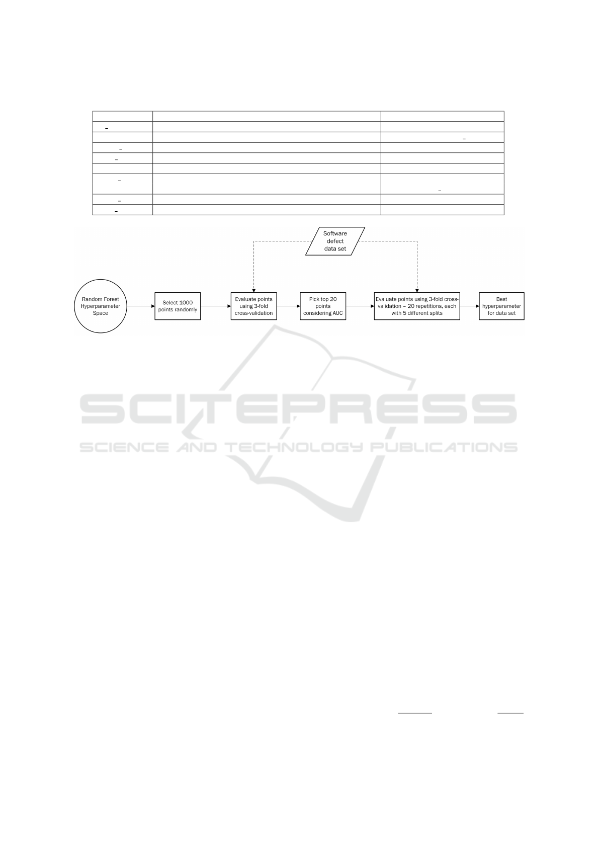
Table 2: Hyperparameters of the Random Forest algorithm and the values used for tuning.

Parameter Description Values considered for tuning

n estimators number of trees to build 50, 75, 100, 150, 200

criterion function used to measure the quality of the split gini, etropy, log loss

max depth maximum depth of a tree 3, 5, 7, 9

max features number (fraction) of features to check for the best split log2, sqrt, 0.25, 0.5, 0.75, 0.95

bootstrap whether bootstrap sampels are used for building the trees True, False

class weight weights assigned for the classes None, balanced,

balanced subsample

ccp alpha parameter used for determining which subtree to prune 0, 0.01, 0.02, 0.03, 0.04

max samples the maximum fraction of samples to use if bootstrap is True 0.5, 0.6, 0.7, 0.8, 0.9

Figure 1: Steps of the hyperparameter tuning process.

perparameter space, several runs for that point should

be executed. In order to balance the total run time and

the exploration of the hyperparameter space, we have

decided to use a two-step parameter tuning process,

which is presented on Figure 1.

For each of the 16 data sets and each of the three

representations, ﬁrst we have selected 1000 random

hyperparameter points and evaluated them using a

single run of a 3-fold cross validation on the current

data set using the AUC measure. This is called ran-

dom search-based hyperparameter tuning and is an

alternative for grid search which was shown in (Tan-

tithamthavorn et al., 2019) to perform just as well as

grid search for SDP.

In the second step of the process, the 20 points

with the highest AUC from the ﬁrst step were selected

and re-evaluated. The 3-fold cross validation was re-

peated 20 times and for each repetition 5 different ran-

dom splittings into the 3-folds were considered. Con-

sequently, for every point, we had the value of AUC

for 100 evaluations. The average of these values was

considered to be the evaluation value of that hyperpa-

rameter point. Finally, the point with the highest AUC

was selected as the best hyperparameter for the given

data set and representation.

3.3.3 Evaluation Methodology

In order to evaluate the performance of the three su-

pervised models, when fed with different vectorial

representations, scaled in [0,1] using Min-Max nor-

malization, we employed the following evaluation

methodology. For FastAI and MLP the data was split

into 70% train, 10% validation (for early stopping)

and 20% test sets. For RF there was no early stopping,

so the data was split into 80% train and 20% test set.

In order to get consistent results, 30 experiments with

different splits had been performed.

During this evaluation process, the confusion ma-

trix for the binary classiﬁcation task has been com-

puted for each of the 30 testing subsets. Based on the

confusion matrix (TP - number of true positives, FP -

number of false positives, TN - number of true neg-

atives and FN - number of false negatives), the Area

under the ROC curve (AUC) has been computed as a

performance indicator. The reported values have been

averaged over the 30 experiments.

We considered AUC as a performance evalua-

tion measure because the SDP literature reveals that

AUC is particularly suitable for evaluating the per-

formance of the software defect classiﬁers (Fawcett,

2006). In general, the AUC measure is employed for

approaches that yield a single value, which is then

converted into a class label using a threshold. Thus,

for each threshold value, the point (1 − Spec, Sens) is

represented on a plot and the AUC is computed as

the area under this curve. For the approaches where

the direct output of the defect classiﬁer is the class la-

bel, there is only one (1 − Spec, Sens) point, which

is linked to the (0, 0) and (1, 1) points. The AUC

measure represents the area under the trapezoid and is

computed as the mean of sensitivity (Sens) and speci-

ﬁcity (Spec): AUC =

Sens+Spec

, where Sens =

T P

T P+FN

ICSOFT 2023 - 18th International Conference on Software Technologies

190

and Spec =

T N

T N+FP

. AUC ranges from 0 to 1. Higher

values indicate better classiﬁcation performance.

4 RESULTS AND DISCUSSION

4.1 Difﬁculty Analysis

In order to answer our ﬁrst research question pre-

sented in Section 1, we have ﬁrst computed the posi-

tive and negative difﬁculty of the data sets generated

by using each of the three embeddings for each of the

16 versions. The computation of the difﬁculty values

was performed according to Section 3.3.1.

The difﬁculty values computed for the defective

class can be seen on Figure 2, while the ones for the

non-defective class are represented on Figure 3.

By analyzing Figure 2, where, for a clearer pre-

sentation of the differences, the y-axis labels start

from 0.5, we can observe that the difﬁculty for the

positive class is quite high. Most values are around

0.6-0.7, the minimum is 0.551 and for some versions

and representations it can be as high as 0.83. This

means that, on average, around two thirds of the de-

fective instances are closer to a non-defective instance

than to a defective one, which makes the correct pre-

diction of defective entities a very difﬁcult task.

If we compare the values for different embed-

dings, we can see that for 12 versions out of 16,

the Graph2Vec representation leads to a lower dif-

ﬁculty than the other two. This suggests that the

Graph2Vec embedding captures structural informa-

tion which could be relevant for identifying defects.

However, analyzing Figure 3 that represents the

difﬁculty for the negative class, besides observing that

the values are a lot smaller, most of them below 0.1,

we can also observe that this time the Doc2Vec + LSI

embedding is the one that produces lower difﬁcul-

ties. This suggests that the Doc2Vec + LSI embed-

ding manages to better capture the characteristics of

the non-defective entities.

The fact that one representation produces lower

difﬁculty values for the positive class while the other

produces lower difﬁculty values for the negative class

suggests that the two representations capture different

aspects of the software entities and thus conﬁrm our

intuition that they complement each other by catch-

ing together both semantic and syntactic information

underlying the source code.

4.2 Supervised Analysis

For performing the comparative analysis from the per-

spective of supervised learning, we have run the three

classiﬁcation algorithms presented in Section 3.3.2 on

all 16 versions of Calcite fed with the three embed-

dings proposed in Section 3.2.

The AUC values for FastAI, MLP and RF are de-

picted on Figures 4, 5 and 6, respectively. All the

AUC values are the averages for the 30 runs, as pre-

sented in Section 3.3.3. While we did not put them

on the ﬁgures to avoid visual overcrowding, we have

computed the 95% conﬁdence intervals (CI) for all

AUC values. For FastAI and RF the margin of error

is at most 0.03 (although there is one single case for

RF where it is 0.08), while for MLP it is at most 0.02.

Even if, due to the lack of space, we do not detail

all the numeric results in the current paper, a docu-

ment with the complete values for all algorithms and

all runs is available on Figshare (ﬁg, 2023).

4.2.1 RQ1: The Relative Relevance of

Graph2Vec-Based Embedding

As regards RQ1, considering the FastAI algorithm

(Figure 4), we can see that the Graph2Vec and

Doc2Vec + LSI embeddings lead to quite similar SDP

performance, but almost always (15 cases out of 16)

Doc2Vec + LSI outperforms Graph2Vec. The same

stands if we look at the results of the MLP classiﬁer

(Figure 5): the values are close, but Doc2Vec + LSI

performs better for 14 Calcite versions. When con-

sidering the results of RF (Figure 6), we can notice

that Doc2Vec + LSI is better in only 8 cases. More-

over, there are 4 cases (versions 1.5, 1.6, 1.11 and

1.15) where the AUC values for Doc2Vec + LSI are

a lot lower than the ones for Graph2Vec. This aspect

will be discussed in Section 4.2.3. In conclusion, our

answer for RQ1 is that the Graph2Vec embedding per-

forms similarly to Doc2Vec + LSI, but in most cases,

irrespectively of the classiﬁcation algorithm used, it

is outperformed by Doc2Vec + LSI.

4.2.2 RQ2: The Potency of Combining Doc2Vec,

LSI and Graph2Vec-Based Embeddings

In order to answer RQ2, we look at Figures 4, 5, and

6 again. We can see that, for all three algorithms, in

12 out of 16 cases, the Doc2Vec + LSI + Graph2Vec

is the best-performing one. This is summarized on

Figure 7. To further verify if the Doc2Vec + LSI +

Graph2Vec representation indeed captures informa-

tion about the characteristics of defective and non-

defective entities, we have performed an additional

experiment. We run the RF classiﬁer with the best hy-

perparameter selected for each version of the Calcite

software system, but we have randomly shufﬂed the

class labels. In this way, we try to learn from a ran-

dom data set. If the classiﬁer has, on the random data,

Source-Code Embedding-Based Software Defect Prediction

191

Figure 2: Difﬁculty values for the three vectorial representations considering only the defective class.

Figure 3: Difﬁculty values for the three vectorial representations considering only the non-defective class.

results comparable to the ones on the original one, it

suggests that only random noise has been learnt. We

have used the same methodology as for the other ex-

periments, 20% of data being randomly selected for

testing (the labels being randomly shufﬂed) and for

each version the experiment being repeated 30 times

to account for randomness in the classiﬁer. The aver-

age AUC values obtained for the 16 versions are be-

tween 0.478 and 0.521, so a lot below the AUC values

for the original data set, which are above 0.71. This

conﬁrms that the Doc2Vec + LSI + Graph2Vec em-

bedding captures aspects carrying discriminative in-

formation that enables differentiating between defec-

tive and defect-free software entities.

Consequently, our answer for RQ2 is that the

Graph2Vec and Doc2Vec + LSI embeddings improves

the performance of the SDP model.

ICSOFT 2023 - 18th International Conference on Software Technologies

192

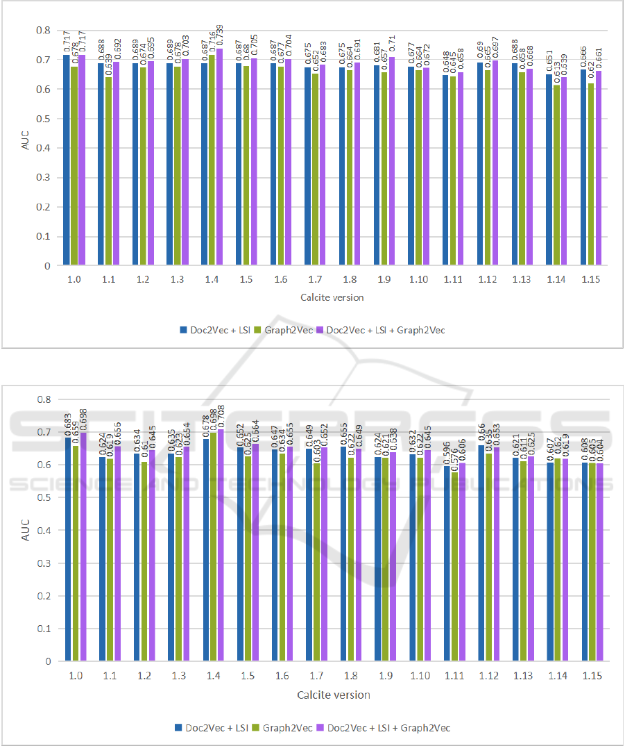
Figure 4: AUC values computed for the experimental evaluation of the FastAI classiﬁer and the three studied embeddings.

Figure 5: AUC values computed for the experimental evaluation of the MLP classiﬁer and the three studied embeddings.

4.2.3 RQ3: FastAI Versus Tuned Random

Forest as Defect Prediction Models

Our third research question is related to the perfor-

mance of the hyperparameter-tuned RF compared to

FastAI, the deep learning classiﬁer.

To answer this question, we have looked at our

results from a different perspective. Instead of com-

paring the performance obtained by the same classi-

ﬁer for different embeddings, we have compared the

Source-Code Embedding-Based Software Defect Prediction

193

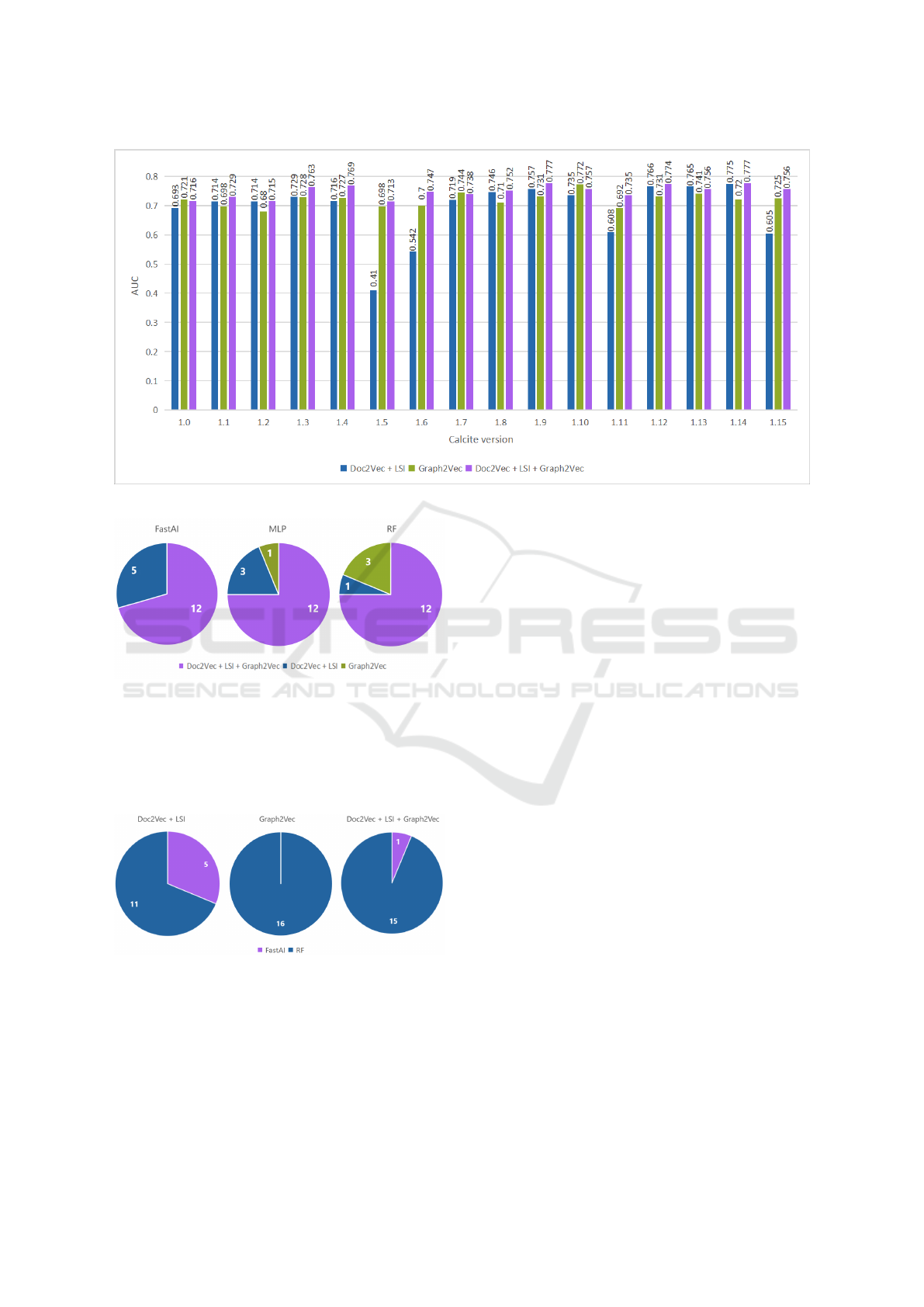
Figure 6: AUC values computed for the experimental evaluation of RF classiﬁer and the three studied embeddings.

Figure 7: The number of best-performing vectorial repre-

sentations for the 16 versions of the Calcite software sys-

tem, for each classiﬁcation algorithm.

performance of the two classiﬁers for the same em-

beddings. Due to lack of space, we only include the

summary of the comparisons, depicted on Figure 8.

Figure 8: The number of best-performing classiﬁers for the

16 versions of the Calcite software system, for each embed-

ding.

As illustrated in Figure 8, the tuned RF classi-

ﬁer outperforms FastAI for all representations. This

conﬁrms the conclusions presented in (Fu and Men-

zies, 2017) and (Majumder et al., 2018), claiming that

properly tuned simpler models can outperform deep

learning models. In order to check that the parameter

tuning indeed matters, we have repeated the experi-

ments for the Doc2Vec + LSI + Graph2Vec represen-

tation (since, according to the conclusions of RQ2,

this is the best-performing embedding) considering

the default parameters of RF from scikit-learn. The

results were all less than 0.55, which is signiﬁcantly

lower than the AUC values achieved for the tuned RF,

that are all above 0.71.

As presented in Section 3.3.2 we have used the

random search-based parameter tuning approach for

RF. The previous experiment demonstrated that de-

fault parameters perform quite poor on the Doc2Vec

+ LSI + Graph2Vec embedding, so we have decided

to look at the initially generated 1000 hyperparameter

points, to see how varied their AUC values are. For all

data sets and representations there were hyperparame-

ter points with an AUC value of 0 (at least 97, at most

462) and a lot of points with an AUC value below 0.5

(at least 162 and at most 995). Actually, there were 4

versions of the Calcite data set, for which there was an

exceptionally high number of hyperparameter points

with an initial AUC value below 0.5: version 1.5 (995

points), 1.6 (903), 1.11 (844) and 1.15 (929). On Fig-

ure 6 we can see that these are exactly the versions

with an AUC value a lot less than the other versions

and representations. This is probably the result of a

random search which produced a lot of hyperparame-

ter points with very poor performance. This suggests

that in some cases, random search might not gener-

ate good enough points, and probably the number of

points should be increased in such cases.

Our ﬁndings about how much parameter tuning

ICSOFT 2023 - 18th International Conference on Software Technologies

194

matters for RF are different from the ﬁndings of Tan-

tithamthavorn (Tantithamthavorn et al., 2019), who

concluded that RF is not sensitive to hyperparame-

ter tuning (although they only tuned the parameter

denoting the number of trees). The reason for this

discrepancy might be given by the difference in the

considered features: we have used embeddings learnt

from the source code, while in (Tantithamthavorn

et al., 2019) structural, complexity and size metrics

are used. There is another observation regarding RFs

in (Tantithamthavorn et al., 2019): they are not among

the top-performing classiﬁers. In our study, RFs had

the best performance, but we compared only 3 ap-

proaches and only the parameters of RF were tuned,

while Tantithamthavorn et al. compared 26 classiﬁers,

so it is possible that even better performance can be

achieved by considering other classiﬁers.

Consequently, our answer for RQ3 is that, for our

data sets, the RF classiﬁer with the best hyperparam-

eter setting outperforms FastAI in most cases. Never-

theless, there were 4 identiﬁed cases when the random

search parameter tuning approach could not identify

good enough parameters and in these cases the per-

formance of FastAI was better than that of RF.

4.2.4 Statistical Tests

In order to test if the conclusions of the three re-

search questions are statistically signiﬁcant, we have

performed some statistical tests. RQ1 and RQ2 fo-

cus on the comparison of different source code em-

beddings, so we have ﬁrst considered the 48 AUC

values for each source code embedding (16 values

for each classiﬁer). According to the Kolmogorov-

Smirnov test (with Lilliefors’ method) all three vari-

ables (i.e. set of AUC values for code embeddings)

are normally distributed so we have used a one-way

repeated measures ANOVA test. Mauchly’s test indi-

cated that the assumption of sphericity had been vio-

lated, therefore degrees of freedom were corrected us-

ing Greenhouse-Geisser estimates of sphericity. The

results of ANOVA show that the AUC values for

the three embeddings differ signiﬁcantly. Post hoc

tests revealed that the Doc2Vec + LSI + Graph2Vec

representation has signiﬁcantly higher AUC values

than both other representations. However, there is

no signiﬁcant difference between Doc2Vec + LSI and

Graph2Vec embeddings.

For RQ3, we have compared the 16 AUC values

for the FastAI and RF classiﬁer for the Doc2Vec +

LSI + Graph2Vec embedding. Since the Kolmogorov-

Smirnov test showed that both variables are normally

distributed, we used a one-way repeated measures

ANOVA again (even if we had only two variables)

whose results show that the AUC values for RF are

signiﬁcantly higher than those for FastAI.

Consequently, we can conclude that the results for

RQ2 and RQ3 are statistically signiﬁcant.

5 CONCLUSIONS

In this paper, we proposed using Graph2Vec embed-

ding as a new representation of software entities in

defect prediction models. Results from several exper-

imental analyses have conﬁrmed the relevance of the

proposed representation in identifying defect prone-

ness. Additionally, when using Graph2Vec embed-

ding in conjunction with Doc2Vec and LSI embed-

dings, their complementarity boosts the defect pre-

diction performance. In our comparative analysis, we

have employed three classiﬁcation models, including

the FastAI deep learning model and a hyperparame-

ter tuned Random Forest, the latter outperforming the

former, which reveals the potency of hyperparameter

optimisation in the case of software defect predictors.

To reinforce the conclusions of our present study

we aim to further extend the experimental analyses

by considering additional open-source software sys-

tems and machine learning models. We also envision

investigating the potency of CodeBERT and graph-

CodeBERT for SDP and to reliably compare it to that

of our current approach.

ACKNOWLEDGEMENTS

This work was supported by a grant of the Min-

istry of Research, Innovation and Digitization,

CNCS/CCCDI – UEFISCDI, project number PN-III-

P4-ID-PCE-2020-0800, within PNCDI III.

REFERENCES

(2017). The seacraft repository of empirical software engi-

neering data.

(2023). Source-code embedding-based software defect pre-

diction - data sets and detailed results. https://ﬁgshare.

com/s/d5a7e8126ccd94181511.

Aladics, T., J

asz, J., and Ferenc, R. (2021). Bug predic-

tion using source code embedding based on Doc2Vec.

In Computational Science and Its Applications, pages

382–397.

Begoli, E., Camacho-Rodr

ıguez, J., Hyde, J., Mior, M. J.,

and Lemire, D. (2018). Apache Calcite: A founda-

tional framework for optimized query processing over

heterogeneous data sources. In Proc. of the Interna-

tional Conf. on Management of Data, page 221–230.

Source-Code Embedding-Based Software Defect Prediction

195

Breiman, L. (2001). Random forests. Machine Learning,

45:5–32.

Dam, H. K., Pham, T., Ng, S. W., Tran, T., Grundy, J.,

Ghose, A., Kim, T., and Kim, C.-J. (2018). A deep

tree-based model for software defect prediction.

Deerwester, S. C., Dumais, S. T., Landauer, T. K., Furnas,

G. W., and Harshman, R. A. (1990). Indexing by latent

semantic analysis. Journal of the American Society for

Information Science, 41:391–407.

Fawcett, T. (2006). An introduction to ROC analysis. Pat-

tern Recognition Letters, 27(8):861–874.

Fu, W. and Menzies, T. (2017). Easy over hard: A case

study on deep learning. In Proc. of the Joint Meeting

on Foundations of Software Engineering, page 49–60.

Herbold, S., Trautsch, A., Trautsch, F., and Ledel, B.

(2022). Problems with szz and features: An empirical

study of the state of practice of defect prediction data

collection. Empirical Software Engineering, 27(2).

Howard, J. et al. (2018). fastai. https://github.com/fastai/

fastai.

Le, Q. V. and Mikolov, T. (2014). Distributed represen-

tations of sentences and documents. Computing Re-

search Repository (CoRR), abs/1405.4:1–9.

Li, J., He, P., Zhu, J., and Lyu, M. R. (2017). Software de-

fect prediction via convolutional neural network. In

IEEE International Conf. on Software Quality, Relia-

bility and Security, pages 318–328.

Majumder, S., Balaji, N., Brey, K., Fu, W., and Menzies,

T. (2018). 500+ times faster than deep learning: A

case study exploring faster methods for text mining

stackoverﬂow. In Proceedings of the 15th Interna-

tional Conference on Mining Software Repositories,

MSR ’18, page 554–563.

Malhotra, R. (2015). A systematic review of machine learn-

ing techniques for software fault prediction. Applied

Soft Computing, 27:504 – 518.

Matloob, F., Ghazal, T. M., Taleb, N., Aftab, S., Ahmad,

M., Khan, M. A., Abbas, S., and Soomro, T. R.

(2021). Software defect prediction using ensemble

learning: A systematic literature review. IEEE Access,

9:98754–98771.

Miholca, D. and Onet-Marian, Z. (2020). An analysis of

aggregated coupling’s suitability for software defect

prediction. In 2020 22nd International Symposium on

Symbolic and Numeric Algorithms for Scientiﬁc Com-

puting, pages 141–148. IEEE Computer Society.

Miholca, D.-L. and Czibula, G. (2019). Software defect

prediction using a hybrid model based on semantic

features learned from the source code. In Knowledge

Science, Engineering and Management: 12th Interna-

tional Conference, Part I, page 262–274.

Miholca, D.-L., Czibula, G., and Tomescu, V. (2020).

Comet: A conceptual coupling based metrics suite for

software defect prediction. Procedia Computer Sci-

ence, 176:31–40.

Miholca, D.-L., Tomescu, V.-I., and Czibula, G. (2022). An

in-depth analysis of the software features’ impact on

the performance of deep learning-based software de-

fect predictors. IEEE Access, 10:64801–64818.

Narayanan, A., Chandramohan, M., Venkatesan, R., Chen,

L., Liu, Y., and Jaiswal, S. (2017). Graph2vec: Learn-

ing distributed representations of graphs.

Neto, E. C., da Costa, D. A., and Kulesza, U. (2018).

The impact of refactoring changes on the szz algo-

rithm: An empirical study. 2018 IEEE 25th Inter-

national Conference on Software Analysis, Evolution

and Reengineering (SANER), pages 380–390.

Pan, C., Lu, M., and Xu, B. (2021). An empirical study on

software defect prediction using CodeBERT model.

Applied Sciences, 11(11).

Pedregosa, F., Varoquaux, G., Gramfort, A., Michel, V.,

Thirion, B., Grisel, O., Blondel, M., Prettenhofer,

P., Weiss, R., Dubourg, V., Vanderplas, J., Passos,

A., Cournapeau, D., Brucher, M., Perrot, M., and

Duchesnay, E. (2011). Scikit-learn: Machine learning

in Python. Journal of Machine Learning Research,

12:2825–2830.

Reh

rek, R. and Sojka, P. (2010). Software framework for

topic modelling with large corpora. In Proceedings of

the LREC 2010 Workshop on New Challenges for NLP

Frameworks, pages 45–50. ELRA.

Rozemberczki, B., Kiss, O., and Sarkar, R. (2020). Karate

Club: An API Oriented Open-source Python Frame-

work for Unsupervised Learning on Graphs. In Proc.

of the ACM International Conf. on Information and

Knowledge Management, page 3125–3132. ACM.

Sayyad, S. and Menzies, T. (2015). The PROMISE reposi-

tory of software engineering databases. School of In-

formation Technology and Engineering, University of

Ottawa, Canada.

Sikic, L., Kurdija, A. S., Vladimir, K., and Silic, M. (2022).

Graph neural network for source code defect predic-

tion. IEEE Access, 10:10402–10415.

Tantithamthavorn, C., McIntosh, S., Hassan, A. E., and

Matsumoto, K. (2019). The impact of automated

parameter optimization on defect prediction models.

IEEE Trans. on Software Eng., 45(7):683–711.

Uddin, M. N., Li, B., Ali, Z., Kefalas, P., Khan, I., and

Zada, I. (2022). Software defect prediction employ-

ing BiLSTM and BERT-based semantic feature. Soft

Computing, 26:1–15.

Wang, S., Liu, T., Nam, J., and Tan, L. (2020). Deep se-

mantic feature learning for software defect prediction.

IEEE Trans. on Software Eng., 46(12):1267–1293.

Wang, S., Liu, T., and Tan, L. (2016). Automatically learn-

ing semantic features for defect prediction. In Proc. of

the Int. Conf. on Software Eng., pages 297–308.

Zhang, D., Tsai, J., and Boetticher, G. (2007). Improving

credibility of machine learner models in software en-

gineering. In Advances in Machine Learning Applica-

tions in Software Engineering, pages 52–72.

ICSOFT 2023 - 18th International Conference on Software Technologies

196