A Comparison of the Dynamic Temperature Responses of Two

Different Heat Exchanger Modelling Approaches in Simulink

Simscape for HVAC Applications

Samuel F. Fux, Babak Mohajer and Stefan Mischler

Belimo Automation AG, Brunnenbachstrasse 1, 8640 Hinwil, Switzerland

Keywords: HVAC, Heat Exchanger, Dynamic Response, Dynamic Simulation Models, MATLAB/Simulink/Simscape.

Abstract: In the HVAC industry, the dynamic temperature response of water-to-air heat exchangers is of particular

importance for control system design. In this paper, the dynamic temperature responses of two established

thermal dynamic modelling approaches for heat exchangers, the single-segment modelling using the

effectiveness-NTU method and the multi-segment modelling, are investigated. Both approaches are validated

against experimental data recorded with two different heat exchangers used in HVAC systems. A quasi-static

analysis reveals minor differences between the results of the two models considered. The dynamic analysis is

performed with varying inlet conditions. First results show that the single-segment model may fail to properly

reproduce the water outlet temperature dynamics of a heat exchanger under certain conditions. In the tests

performed in this study, however, the multi-segment model captures the relevant dynamics. The influence of

this difference in the dynamic behaviour of the single-segment model on the model-based development of

control algorithms is subject of future studies.

1 INTRODUCTION

In heating, ventilation, and air conditioning (HVAC)

systems in buildings, typically, water-to-air heat

exchangers are used to condition the temperature of

the supply air. To increase the occupant comfort in

the building and to decrease the energy use of the

HVAC system, optimal operation of the heat

exchanger is crucial. The development and testing of

new control algorithms for the operation of HVAC

heat exchangers can be simplified and accelerated by

using building simulation environments with an

appropriate dynamic model of the heat exchanger

(Zhou and Braun, 2004). An appropriate dynamic

heat exchanger model must be able to accurately

predict the water and air outlet temperatures not only

during steady state operation but also during

transients when the inlet conditions are changing.

Furthermore, it is important that the model is accurate

across the entire operating range and not only at full

load.

In the past decades, authors presented different

approaches for modelling the dynamic temperature

behaviour of HVAC water-to-air heat exchangers for

the purpose of control performance analysis. For

instance, (Underwood, 1990) developed a heat

exchanger model based on single energy balance

equations for the water and the air side, respectively.

The same lumped parameter approach is also

employed by, e.g., (Zajic, Larkowski, Sumislawska,

Burnham, and Hill, 2011) and (Afram and Janabi-

Sharifi, 2015).

In (Zhou and Braun, 2004), a model is presented

where the heat exchanger is divided into a series of

basic elements. Each basic element represents a

cross-flow finned tube. Then, a transient model for

the basic element is introduced, which considers

energy storage in the water and in the tube and fin

material. This approach of discretising the heat

exchanger into multiple smaller elements is adopted

by (Jie and Braun, 2016).

A completely different approach is introduced by

(Anderson, 2001), who proposes a linear model at an

operating point. This model is formed by combining

several first-order transfer functions and time delays.

The goal of this paper is to assess the suitability of

two popular modelling approaches for testing control

algorithms. For that purpose, two different heat

exchanger models are compared with temperature

measurement data from real heat exchangers. Both

Fux, S., Mohajer, B. and Mischler, S.

A Compar ison of the Dynamic Temperature Responses of Two Different Heat Exchanger Modelling Approaches in Simulink Simscape for HVAC Applications.

DOI: 10.5220/0012132300003546

In Proceedings of the 13th International Conference on Simulation and Modeling Methodologies, Technologies and Applications (SIMULTECH 2023), pages 417-424

ISBN: 978-989-758-668-2; ISSN: 2184-2841

 2023 by SCITEPRESS – Science and Technology Publications, Lda. Under CC license (CC BY-NC-ND 4.0)

417

models are implemented in the MATLAB®

Simulink® simulation environment using the

Simscape modelling language (The MathWorks, Inc.,

2023a).

The paper is structured as follows: In Section 2,

an overview on the structure of HVAC heat

exchangers is provided. Section 3 introduces the two

models considered in this study. The comparison of

the two models with measurement data is shown in

Section 4. Finally, the conclusions of this study are

summarized in Section 5.

2 STRUCTURE OF HVAC HEAT

EXCHANGERS

Heat exchangers are usually characterized in one of

the four major construction types: tubular, plate-type,

extended surface, and regenerative heat exchangers

(Shah and Sekulić, 2003).

One of the commonly used water-to-air heat

exchanger types in the HVAC industry are the

extended surface exchangers. To compensate the low

heat transfer coefficient on the air side and to increase

the efficiency, fins are being used to extend the

surface area up to 5 – 12 times the primary surface

area (Shah and Sekulić, 2003), see Figure 1.

Air Flow

Figure 1: Finned tubular cross flow heat exchangers with

both fluids unmixed.

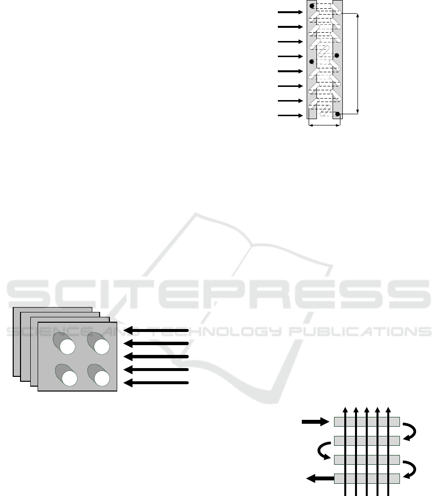
This paper focuses on the modelling of fin and

tube heat exchangers and their circuiting pattern. The

circuiting pattern of the water tubes is one of the

important aspects which influences the performance

of the heat exchanger. The number of tube rows mark

the depth and the number of tubes in each row mark

the height of the heat exchanger. Furthermore, the

number of circuits in a heat-exchanger is defined by

the number of tubes that are fed by the supply header

(Campbell Sevey, 2023). As an example, a quarter

circuit heat exchanger with two feeds is shown in

Figure 2.

Height: 8 Tubes

Depth: 4 Rows

Supply

Return

Air Flow

Figure 2: Quarter circuit heat-exchanger (adapted from

(Campbell Sevey, 2023)).

Determining the proper number of circuits, the

speed of the fluid in the tubes as well as the resulting

pressure drop can be controlled. This both aspects

have a direct impact on the heat transfer efficiency of

the heat exchanger (Campbell Sevey, 2023).

While talking about the circuiting it is important

to also consider how often the air crosses the inner

tubes perpendicularly (number of passes).

Common flow arrangements of water-to-air heat

exchangers are: (VDI Gesellschaft Verfahrenstechnik

und Chemieingenieurwesen, 2019):

• multi-row, single-pass

• multi-row, multi-pass

• multi-row, two-pass

In Figure 3, a flow scenario with 4 rows and 4 passes

is illustrated. In this flow arrangement the tube rows

are connected in series with alternating flow

directions in each row. The outside air crosses the

tubes 4 times.

Air Flow

Liquid Flow

Figure 3: Crossflow definition for 4 rows and 4 passes

(adapted from (VDI Gesellschaft Verfahrenstechnik und

Chemie-ingenieurwesen, 2019)).

Considering the above-mentioned aspects, it is

crucial to take the circuiting arrangement into account

when modelling a heat exchanger.

SIMULTECH 2023 - 13th International Conference on Simulation and Modeling Methodologies, Technologies and Applications

418

3 HEAT EXCHANGER MODELS

As mentioned in the introduction, there exists a

variety of dynamic models to predict the temperature

behaviour of HVAC water-to-air heat exchangers.

However, these models are usually based on one of

the following basic approaches:

- Simple single-segment models, in which the water

and air sides are entirely lumped into single

thermal capacities each.

- Detailed multi-segment models, in which the heat

exchanger is divided into a fixed number of

smaller segments.

Furthermore, the various models differ in how

detailed they compute the heat transfer between the

water and the air side and if they consider the heat

capacity of the tube and fin material or not.

In this paper, an example of a single-segment

model and an example of a multi-segment model are

evaluated using measurement data. The two models

are presented in the following two subsections.

3.1 Single-Segment Model

The first model considered in this study is the heat

exchanger model provided with the Simscape Fluids

component library (The MathWorks, Inc., 2023b).

Since only one energy conservation equation is

formulated for each of the water and air sides, this

model belongs to the category of single-segment

models.

This model uses the effectiveness-NTU method to

compute the heat transfer between the water and the

air side. It can also consider water condensation on

the air side. However, the thermal capacity of the

tubes and fins are not considered. In addition to the

temperature dynamics, the model also computes the

pressure losses across the heat exchanger. Please refer

to (The MathWorks, Inc., 2023c) for a detailed

description of the model.

Important input parameters required by the model

include the following: flow arrangement and

geometries, length of the tubes, tube outer diameter,

number of rows, number of tubes per row,

longitudinal and transverse tube spacing, fouling

factors, total fin surface area, and constant fin

efficiency. The model does not require the input of

parameter values which need to be identified using

measurement data (e.g., convective heat transfers

coefficients).

3.2 Multi-Segment Model

The second model used in this study is a multi-

segment model developed by the authors.

The development of this model is based on the

assumptions typical for this type of model (e.g.,

(Zhou and Braun 2004) or (Mathisen, Morari, and

Skogestad, 1994)):

• all segments have the same size,

• ideal mixing of the water in each segment,

• ideal mixing of the air in each segment,

• the tube and fin material separating water and air

side have a uniform temperature distribution in

each segment,

• heat conduction between adjacent segments is

neglected,

• heat losses from the heat exchanger to the

surroundings are not considered.

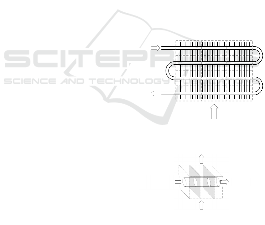
The division of a heat exchanger into smaller

segments is exemplified in Figure 4. The schematic

of one segment of the multi-segment model is then

depicted in Figure 5.

Water flow

Air flow

Figure 4: Example of the division of a heat exchanger into

multiple smaller segments.

Figure 5: Schematic of the i-th segment of the multi-

segment heat exchanger model.

𝑇

,





𝑡



𝑇

,





𝑡



𝑚









𝑡



𝑇

,





𝑡



𝑇

,





𝑡



𝑚



,



𝑡



A Comparison of the Dynamic Temperature Responses of Two Different Heat Exchanger Modelling Approaches in Simulink Simscape for

HVAC Applications

419

In this model, energy conservation equations are

formulated for the water side, the air side and for the

metal mass. Obviously, the energy conservation

equations account for the fluid flows through the

segment and the convective heat transfers between

the fluids and the metal surfaces.

The required geometric dimensions of the heat

exchanger are computed in the model as presented in

(Réz, 2004) and (Vetter, 2014). The fin efficiency of

the continuous plate fins is calculated considering an

equivalent fin radius as given in (Perrotin and Clodic,

2003).

Finally, the convective heat transfer coefficient on

the air side is computed using the equivalent diameter

𝐷



and the appropriate empiric correlations for the

Nusselt number (Réz, 2004).

The multi-segment model is implemented in

Simulink® using the Simscape modelling language,

too. Except for the calculation of the convective heat

transfer coefficient on the air side, the

implementation of the model is based on component

models available in the Simscape Foundation library.

Consequently, the model also considers water

condensation.

This model requires similar input parameters as

the single-segment model presented above. However,

it must be mentioned that the fin efficiency is not

required since it is calculated online in the model.

4 TEST RESULTS

The two models presented above are evaluated using

measurement data recorded with one heating and one

cooling heat exchanger. Some properties of the two

heat exchangers are given in Table 1 and Table 2,

respectively.

The heating heat exchanger is installed in a test rig

that is located in an indoor room. Therefore, the inlet

air to the heat exchanger is the same as the room air.

For this reason, the inlet air temperature is

unrealistically high for an HVAC heating application.

However, since the temperature dependency of the air

properties are considered in both models, this is not

deemed to be a problem for the validation of the

models.

On the other hand, the cooling heat exchanger is

installed in a real ventilation system that is used for

the conditioning of a break room in an office building.

Both heat exchangers are equipped with

temperature sensors at the inlet and outlet of the water

side and the air side. For the air temperature sensors,

it must be pointed out that they measure the air stream

temperature only at one location in the air duct.

Therefore, if the air stream does not have a uniform

temperature distribution across the duct cross section,

the accuracy of the temperature measurement must be

challenged.

Table 1: Properties of the heating heat exchanger.

Pro

ert

Value

Height 0.398

Width 0.7

Number of rows 2

Number of tubes

er row 16

Number of circuits 8

Table 2: Properties of the cooling heat exchanger.

Property Value

Height 0.24

Width 0.369

Number of rows 4

Number of tubes

er row 6

Number of circuits 1

Furthermore, there are water volume flow rate

meters in the connecting water pipes of both heat

exchangers. Additionally, measurement data of the

air volume flow rate through the cooling heat

exchanger is available. The heating heat exchanger is

not equipped with a sensor measuring the air volume

flow rate. Therefore, the air volume flow rate must be

estimated based on an energy balance across the heat

exchanger.

For the evaluation, various measurement data

sequences are recorded with the heat exchangers. The

recorded measurement data of the inlet conditions,

i.e., water and air inlet temperatures and water and air

volume flow rates, is then used as inlet conditions

during the simulations with the two models. Finally,

the simulated outlet temperatures are compared with

the measured outlet temperatures.

In the so-called quasi-static tests, the water

volume flow rate through the heat exchangers is

slowly ramped up and down to avoid the excitation of

dynamics in the heat exchangers. The other inlet

conditions are kept as constant as possible during the

recording of these measurement sequences. These

quasi-static tests are used to assess the accuracy of the

models across a wide range of operating points. For

assessing the ability of the models to correctly capture

the temperature dynamics, tests with fast varying inlet

conditions are used. These tests are called dynamic

tests in the following.

The comparison of the heat exchanger models

with the measurement data of the quasi-static and the

dynamic tests are shown in the following two

subsections.

SIMULTECH 2023 - 13th International Conference on Simulation and Modeling Methodologies, Technologies and Applications

420

4.1 Quasi-Static Tests

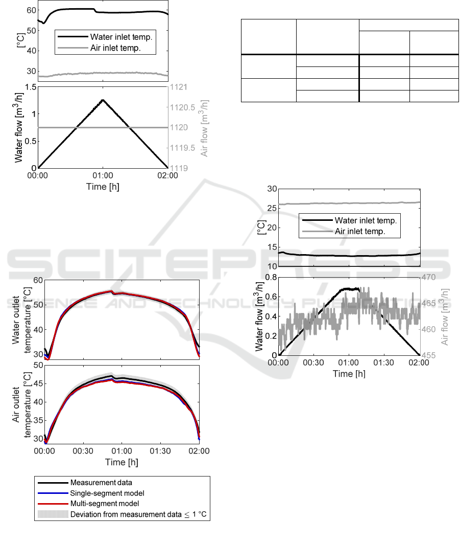
The inlet conditions during the quasi-static test with

the heating heat exchanger are shown in Figure 6.

Figure 6: Inlet conditions for the quasi-static test with the

heating heat exchanger.

The comparison of the two models with the

measurement data of the water and air outlet

temperatures is then plotted in Figure 7.

Figure 7: Comparison of both models with measurement

data from the quasi-static test with the heating heat

exchanger.

In addition, the root mean squared errors

(RMSEs) between the measured and the simulated

water and air outlet temperatures are listed in Table 3.

Table 3: Root mean squared errors of both models for the

quasi-static tests.

Heat

exchanger

Outlet

temperature

Model

Single-

segment

Multi-

segment

Heating

Water 0.68 °C 0.83 °C

Air 0.77 °C 0.78 °C

Cooling

Water 0.25 °C 0.34 °C

Air 0.71 °C 0.53 °C

Figure 8 shows then the inlet conditions for the

quasi-static test with the cooling heat exchanger and

the corresponding comparison of the two models with

the measured outlet temperatures is shown in

Figure 9. The RMSEs of both models for this test are

given in Table 3, too.

Figure 8: Inlet conditions for the quasi-static test with the

cooling heat exchanger.

These results show that both models can

accurately predict the water outlet temperature for

quasi-static inlet conditions across a wide range of

operating points. During most of the time, the

deviation from the measured water outlet temperature

is smaller than 1 °C for both models. Only at low

water volume flow rates, where the water flow is

modelled to be laminar, the deviation increases to

values above 1 °C. In addition, it is assumed that at

low water volume flow rates the heat losses to the

surroundings are not negligible.

A Comparison of the Dynamic Temperature Responses of Two Different Heat Exchanger Modelling Approaches in Simulink Simscape for

HVAC Applications

421

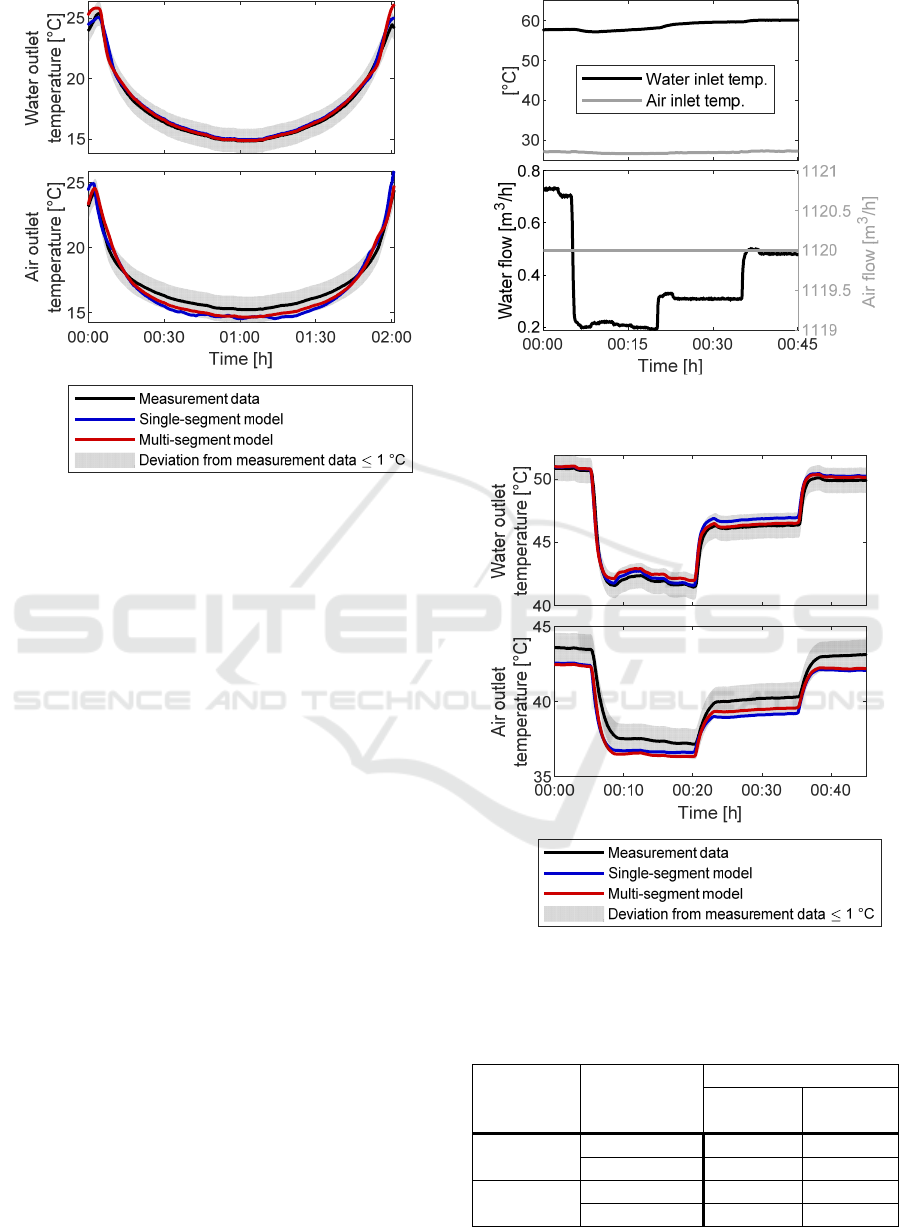
Figure 9: Comparison of both models with measurement

data from the quasi-static test with the cooling heat

exchanger.

For the air outlet temperature, both models seem

to be a bit less accurate. However, it must be

remembered that the accuracy of the air outlet

temperature measurement must be questioned as

explained above.

4.2 Dynamic Tests

To validate the dynamic behaviour of the heat

exchanger models, water volume flow rate step

changes are applied to the heat exchangers. In the

following, the results of these dynamic tests are

presented.

The inlet conditions during a segment of the

dynamic test with the heating heat exchanger and the

corresponding comparison of the two models with the

measured outlet temperatures are shown in Figure 10

and Figure 11, respectively. The RMSEs of the

simulated water and air outlet temperatures for the

complete dynamic test are given in Table 4. Please

note that the dynamics of the temperature sensors are

considered in the simulations.

These results suggest that for this heating heat

exchanger even the simple single-segment model can

capture the relevant dynamics of both the water and

the air outlet temperatures.

Figure 10: Inlet conditions during a segment of the dynamic

test with the heating heat exchanger.

Figure 11: Comparison of both models with measurement

data from the dynamic test with the heating heat exchanger.

Table 4: Root mean squared errors of both models for the

dynamic tests.

Heat

exchanger

Outlet

temperature

Model

Single-

segment

Multi-

segment

Heating

Water 1.12 °C 1.18 °C

Air 0.91 °C 0.85 °C

Cooling

Water 0.34 °C 0.35 °C

Air 0.46 °C 0.47 °C

SIMULTECH 2023 - 13th International Conference on Simulation and Modeling Methodologies, Technologies and Applications

422

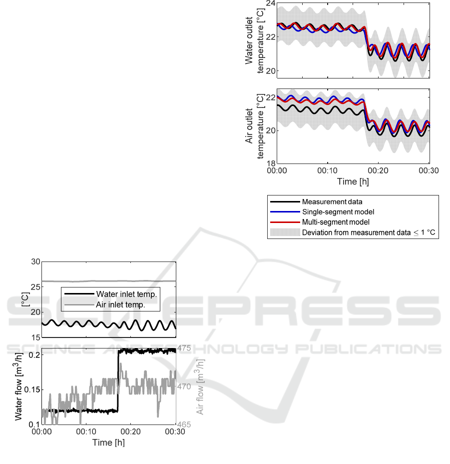
Figure 12 shows then the inlet conditions during a

segment of the dynamic test with the cooling heat

exchanger. The corresponding comparison of the two

models with the measured outlet temperatures is

plotted in Figure 13. The RMSEs of both models for

the complete dynamic test are also provided in

Table 4. These numbers let assume that both models

are equally able to capture the relevant dynamics of

the outlet temperatures. However, as can be seen in

Figure 12, the water inlet temperature is subject to

oscillating disturbances during the test because the

water inlet temperature controller failed to keep a

constant temperature. These disturbances reveal that

the simple single-segment heat exchanger model fails

in this case to always reproduce the dynamics of the

water outlet temperature properly. The comparison of

the simulated water outlet temperature of the single-

segment model with the measurement data in

Figure 13 indicates a time shift of the simulated

response with respect to the measured one for certain

inlet conditions. The multi-segment model, on the

other hand, can capture these dynamics.

Figure 12: Inlet conditions during a segment of the dynamic

test with the cooling heat exchanger.

5 CONCLUSION

The subject of this paper is to investigate two

different approaches of modeling an HVAC water-to-

air heat exchanger and to compare their dynamic

temperature responses for variations in inlet

conditions. For this assessment, measurement data

recorded with one heating and one cooling heat

exchanger are used.

Figure 13: Comparison of both models with measurement

data from the dynamic test with the cooling heat exchanger.

The single-segment model delivered by the

Simscape Fluids component library and the detailed

multi-segment model developed by the authors are

showing overall good accuracy for quasi-static inlet

conditions across a wide range of operating points.

For the heating heat exchanger, both models show

comparable dynamic behavior. Hence, in this case,

the effort for developing the very detailed multi-

segment model and its additional computational

burden during a simulation are not justified.

For the cooling heat exchanger, however, a

noticeable time shift between the water outlet

temperature response of the single-segment model

and the measurement data is observed for certain

variations in inlet conditions, while the multi-

segment model remains accurate. Reasons for this

could be that the multi-segment model additionally

considers the thermal heat capacity of the tube and fin

material and that it represents the transport delay in

the tubes more accurately due to the discretization

approach.

It must be emphasized that the analysis to

substantiate this assumption is not yet complete. To

confirm this initial hypothesis, tests with further

variations of the inlet conditions must be performed.

Finally, so far, the models have been evaluated

only with open loop tests. Additionally, closed loop

studies need to be performed to examine the impact

of the time shift of the single-segment model on

control loop analysis.

A Comparison of the Dynamic Temperature Responses of Two Different Heat Exchanger Modelling Approaches in Simulink Simscape for

HVAC Applications

423

REFERENCES

Afram, A, Janabi-Sharifi, F. (2015). Gray-box modeling

and validation of residential HVAC system for control

system design. Applied Energy, 137, 134 – 150.

Anderson, M. L. (2001). MIMO robust control for heating

ventilating and air conditioning (HVAC) systems

[Master's thesis, Colorado State University].

Campbell Sevey (2023, April 1). A simple guide to coil

circuiting. https://www.campbell-sevey.com/a-simple-

guide-to-coil-circuiting/.

Jie, C., Braun, J. E. (2016). Self-learning backlash inverse

control of cooling or heating coil valves having

backlash hysteresis. International Refrigeration and Air

Conditioning Conference, West Lafayette.

Mathisen, K. W., Morari, M., Skogestad, S. (1994),

Dynamic Models for heat exchangers and heat

exchanger networks. Computers & Chemical

Engineering, 18, 459 – 463.

Perrotin, T., Clodic, D. (2003). Fin efficiency calculation in

enhanced fin-and-tube heat exchangers in dry

conditions. 21st

IIR International Congress of

Refrigeration: Serving the Needs of Mankind,

Washington DC.

Réz, I. (2004). Numerische Untersuchung des luftseitigen

Wärmeübergangs und Druckverlustes in Lamellenrohr-

Wärmeübertragern mit verschiedenen Rohrformen

[Doctoral dissertation, Technische Universität

Bergakademie Freiberg].

Shah, R. K., Sekulić, D. P. (2003). Fundamentals of heat

exchanger design, John Wiley & Sons, Inc.

The MathWorks, Inc. (2023a, April 5). Simscape. Model

and simulate multidomain physical systems. https://

ch.mathworks.com/products/simscape.html.

The MathWorks, Inc. (2023b, April 5). Simscape Fluids.

https://ch.mathworks.com/products/simscape-

fluids.html.

The MathWorks, Inc. (2023c, April 5). Heat exchanger (tl-

ma). https://ch.mathworks.com/help/hydro/ref/

heatexchangertlma.html

Underwood, D. (1990). Modeling and nonlinear control of

a hot-water-to-air heat exchanger. Final report. United

States.

Vetter, C. (2014). Thermodynamische Auslegung und

transiente Simulation eines überkritischen Organic

Rankine Cycles für einen leistungsoptimierten Betrieb

[Doctoral dissertation, Karlsruher Institut für

Technologie].

VDI Gesellschaft Verfahrenstechnik und

Chemieingenieurwesen (2019). VDI heat atlas (12th

edition). Springer.

Zajic, I., Larkowski, T., Sumislawska, M., Burnham, K. J.,

Hill, D. (2011). Modelling of an air handling unit: A

Hammerstein-bilinear model identification approach.

21st International Conference on Systems Engineering,

Las Vegas.

Zhou, X., Braun, J. E. (2004). Transient modeling of chilled

water cooling coils, International Refrigeration and Air

Conditioning Conference, West Lafayette.

SIMULTECH 2023 - 13th International Conference on Simulation and Modeling Methodologies, Technologies and Applications

424