An Open Tool-Set for Simulation, Design-Space Exploration and

Optimization of Supply Chains and Inventory Problems

Tushar Lone

, Lekshmi P.

and Neha Karanjkar

Indian Institute of Technology Goa, India

Keywords:

Supply Chains, Inventory, Discrete-Event Simulation, Python, Meta-Models, Optimization.

Abstract:

This paper presents the design overview and work-in-progress status for InventOpt - a Python-based, open

tool-set for simulation, design space exploration and optimization of supply chains and inventory systems.

InventOpt consists of a Python library of component models that can be instantiated and connected together

to model and simulate complex supply chains. In addition, InventOpt contains a GUI-based tool to assist

the user in planning design of experiments, visualizing the objective functions over a multi-dimensional de-

sign space, building and tuning meta-models and performing meta-model assisted optimization to identify

promising regions in the design space. We present a detailed case study that illustrates the current prototype

implementation, planned features and utility of the tool-set. The case study consists of simulation-based op-

timization of inventory threshold levels in a particular supply chain system with 8 decision parameters. We

present our observations from the case study that lead to design decisions for building InventOpt such as the

choice of the meta-model type, number of simulation measurements for building the meta-model, the choice

of optimizer and the trade-off between computational cost and quality of results. A signiﬁcant aspect of this

work is that each step of the process has been implemented using open Python libraries.

1 INTRODUCTION

A supply chain (SC) is a network of entities (such as

manufacturers, distributors, transporters, warehouses

etc) involved in producing, transporting, storing and

distributing goods and services. The primary goals

in the design of a supply chain are to minimize risk,

maximize net proﬁts and satisfy end-user demands.

(Chopra et al., 2007). Modern supply chains have

complex structures, often spanning multiple conti-

nents and a large set of interconnected entities with

diverse behaviors. Simulation plays a key role in

the design, analysis and optimization of supply chain

systems. While closed-form analytical models suf-

ﬁce to analyze simple supply chains, the use of de-

tailed simulation models becomes necessary to cap-

ture complex behaviors and dependencies between its

components with reasonable accuracy. Simulation al-

lows managers to mitigate risks by evaluating what-

if scenarios and provides a mechanism to identify

bottlenecks and optimize processes for better prof-

https://orcid.org/0000-0003-0008-0429

https://orcid.org/0000-0001-5464-6032

https://orcid.org/0000-0003-3111-1435

its. System Dynamics (SD), Discrete-event Simula-

tion (DES), Monte-Carlo Simulation and Hybrid sim-

ulation are some approaches used for modeling and

studying supply chains. (Mustafee et al., 2021).

Simulation-based optimization is often difﬁcult

owing to the large number of decision variables, the

computational cost of performance estimation using

multiple stochastic simulation runs and non-convex,

black-box objective functions. Since the simulation

model is stochastic, long-run average performance es-

timates (such as the average monthly proﬁt) at a sin-

gle design point can be obtained by averaging the re-

sults over multiple simulation runs with distinct ran-

domization seeds. If each simulation run is assumed

to take a millisecond, the time required for exhaus-

tively evaluating the entire design space will still be

prohibitive. Although there exists no analytical ex-

pression for the objective function or its derivatives in

such problems (black-box optimization), the objective

functions often display low-order trends and can be

mimicked by multi-dimensional polynomial surfaces.

Meta-model based optimization approaches exploits

this aspect. A Meta-model is a function that approx-

imates the detailed simulation model and is compu-

tationally less expensive to evaluate (Barton, 2020).

432

Lone, T., P., L. and Karanjkar, N.

An Open Tool-Set for Simulation, Design-Space Exploration and Optimization of Supply Chains and Inventory Problems.

DOI: 10.5220/0012133300003546

In Proceedings of the 13th International Conference on Simulation and Modeling Methodologies, Technologies and Applications (SIMULTECH 2023), pages 432-439

ISBN: 978-989-758-668-2; ISSN: 2184-2841

 2023 by SCITEPRESS – Science and Technology Publications, Lda. Under CC license (CC BY-NC-ND 4.0)

If X = (x

,...,x

) represents a point in the n-

dimensional design space, and multiple runs of the the

stochastic simulation model estimate some average

performance metric f (X), then the meta-model g(X )

is an (ideally smooth and signiﬁcantly faster to eval-

uate) function which approximates f . It can be con-

structed by measuring f at only a few points in the de-

sign space and performing some form of interpolation

or regression between them. As the number of mea-

surement points increases, the meta-model typically

becomes more and more accurate unless it suffers

from over-ﬁtting (leading to drastic overshoots or os-

cillations in the meta-model surface in-between mea-

sured points). Continuous gradient-based optimiz-

ers can then be applied over the meta-model surface

g to quickly identify promising areas in the design

space for further exploration. Although meta-models

can assist in the optimization process, the process of

choosing the right meta-model type, the number of

data points to build the meta-model and the right op-

timizer can be non-trivial and can signiﬁcantly affect

the results. Response Surface Models (RSM), Ra-

dial Basis Functions, Kriging (Gaussian Process Re-

gression), and Neural Networks (NN) are some meta-

models types that are used in various application do-

mains. Kriging, also known as Gaussian Process Re-

gression (GPR) is a spatial correlation meta-model

(Kleijnen, 2009; Ankenman et al., 2008). It uses a

kernel function to represent the correlation between

different input parameter values. Gaussian kernel,

Radial Basis Function (RBF), and periodic RBF are

some examples of kernel functions used in Kriging).

A Neural Network meta-model is built using a neu-

ral network architecture (for example, a multi-layer

feed-forward network) with the measured points as

training data to learn and mimic the input-output re-

lation. It is then used to approximate the performance

measures of the system at a given point. The pro-

cess of selecting the meta-model type, tuning it and

selecting the right optimizer for optimizing over for it

are nuanced and problem-dependent choices. While

there exist several commercial tools (such as Any-

Logic, FLEXSIM, Arena, IBM Supply Chain solu-

tions), there is a dearth of open libraries in popular

programming languages for supply chain design and

optimization. General-purpose discrete-event simula-

tion frameworks such as Python’s SimPy library (Sim,

2020) can be used for building simulation models of

supply chains. However, validation constitutes a sig-

niﬁcant fraction of model development time. Having

an open library of validated parameterized component

models can be very useful in rapid modeling and de-

sign space exploration. In a similar vein, while there

exist open, general-purpose optimization packages,

an open tool-set speciﬁcally designed for design ex-

ploration and optimization of supply chains can have

wide utility.

This paper presents the design overview and

work-in-progress status of InventOpt - a Python-

based open library and tool-set for supply chain and

inventory systems simulation and meta-model based

optimization. InventOpt primarily consists of a li-

brary of component models for simulating supply

chains. These component models are built using

Python’s SimPy library, and can be instantiated, con-

ﬁgured and connected together to model complex

supply chains. In addition, InventOpt includes a GUI-

based tool for guided design-space exploration, meta-

model tuning and optimization. To make suitable de-

sign choices for InventOpt (such as the meta-model

type, number of measurement points relative to the

size of the design space, and the choice of the op-

timization algorithm) that are speciﬁcally suited for

simulation-based optimization of supply chains, we

present a detailed case study. The case study focuses

on modeling and simulation-based optimization of in-

ventory threshold levels in a particular supply chain

system. The case study illustrates some of the com-

ponents in InventOpt that are already built and those

that can be generalized further, and serves as a val-

idation for the meta-model based approach. Most

importantly, in this case study we perform optimiza-

tions using a wide set of meta-models and optimiz-

ers and compare the solutions to those generated us-

ing a more exhaustive search, as a means of arriv-

ing at design choices for InventOpt. The observations

from the case study lead us to design choices such as

the best meta-model type and parameters, the choice

of optimizer and the number of simulation runs for

a accuracy-versus-computational cost trade-off. The

rest of the paper is organized as follows: in Section 2,

we present a summary of related work and existing

tools for supply chain simulation and optimization.

We then present an overview of InventOpt and dis-

cuss its proposed features and implementation plan in

Section 3. Lastly, Section 4 presents the detailed case

study and a summary of the observations, insights and

conclusions gained from the case study towards the

implementation of InventOpt.

2 RELATED WORK

Anylogic (AnyLogic, 2022), FlexSim (Flexsim,

2022), and Arena (Arena, 2022) are some examples

of popular commercial tools that support supply chain

simulation. AnyLogic and FlexSim also support op-

timization, which is built on top of the OptQuest

An Open Tool-Set for Simulation, Design-Space Exploration and Optimization of Supply Chains and Inventory Problems

433

(OptQuest, 2022) optimization engine. IBM supply

chain solutions (IBM, 2022) is a suite that provides

AI-powered solutions for supply chain optimization.

Among open-source libraries for supply chain sim-

ulation, MiniSCOT (miniSCOT, 2022) is a Python

package for simulating supply chain models that was

developed by Amazon and released as open-source

in 2021 under an Apache licence. However it does

not contain any documentation or usage guidelines

and the latest commit was in 2021. supplychainpy

(Supplychainpy, 2022) is another Python library for

simulating and analyzing supply chains which is pri-

marily meant to replace existing spreadsheet-based

workﬂows. It accepts demand data from a csv ﬁle

and can generate performance metrics based on an-

alytical formulae. It also supports a basic Monte

Carlo simulation that generates normally distributed

demand, based on the historical data in the csv ﬁle.

For design exploration and gaining insights from the

multi-dimensional simulation data, visualization is an

important step. InventOpt will provide a GUI in-

terface to visualise 3D slices of multi-dimensional

data. For a similar purpose, Hypertools (Hypertools,

2022) is an existing Python library for visualizing

high-dimensional data. It also supports dimensional-

ity reduction using the Principal Component Analysis

(PCA) technique.

3 OVERVIEW OF InventOpt

InventOpt is a Python-based, open tool-set targeted

for simulation, design exploration and optimization

of supply chain and inventory problems. This sec-

tion describes the features and components that are

currently implemented (illustrated by the case study

in Section 4) as well as those planned to be imple-

mented in future. InventOpt consists of the following

key components:

• Component Library: An open Python library of

parameterized component models to model the behav-

ior of individual components in supply chains such as

inventory nodes, distributors, manufacturers and de-

mand/customer arrivals. These components can be

instantiated and connected together to model supply

chains with complex structures. In addition, a user

will be able to derive classes from the in-built compo-

nent classes to describe non-standard or custom be-

haviors in a modular and extensible way. Simula-

tion of the instantiated components is performed us-

ing Python’s SimPy DES library.

• Routines for Accuracy-Cost Trade-off: Once a

simulation model has been built, it is necessary to un-

derstand the trade-off between model accuracy and

computational cost. Since the model is stochastic, it is

necessary to perform multiple simulation runs to ob-

tain performance estimates. InventOpt provides rou-

tines for automatically generating the computational

cost versus accuracy trade-off plots at speciﬁed points

in the design space so that a user can predict and bud-

get the computing time for efﬁcient design space ex-

ploration. This is illustrated in our case study pre-

sented in Section 4.

• Tool-set for Design Space Exploration: InventOpt

will provide a GUI interface that would allow a user

to describe the bounds on design variables, scripts to

sample the multi-dimensional design space by per-

forming parallel simulations efﬁciently at multiple

points and visualize the data over a multi-dimensional

space. This step is critical for gaining insight on

the effect of various design variables on performance

measures. It also assists in model validation by al-

lowing the user to visually check for expected trends

and unexpected outliers, possibly pointing to bugs in

the model. In the current implementation (discussed

in Section 4) this functionality is provided via Python

routines and scripts, and a GUI interface will be added

in future.

• Meta-Model Generation Routines: InventOpt

provides a basic GUI interface to build and visual-

ize meta-models for optimization. In future imple-

mentation a GUI will support the user in selecting

the meta-model type, and tuning it by specifying the

number of data points to build the meta-model and the

split between training and test data points for measur-

ing the extent of ﬁt between the original data and the

meta-model. The tool will also provide recommen-

dations or default values for these choices. Once a

meta-model is built, goodness of ﬁt measures (such

as sum-of-squared errors) are reported. The GUI in-

terface also allows the user to visualize the measured

points superimposed on the meta-model. Since the

meta-model is a multidimensional surface, one possi-

ble way is to visualize it as 3D slices with two axes

speciﬁed at a time and the other axes values being

ﬁxed via user input from interactive sliders. Figure

3 shows a screenshot of such a visualization interface

we have implemented for this purpose. Using this in-

terface, the user can select two dimensions at a time

to visualize a 3D slice of the meta-model superim-

posed on the measured simulation data. For the other

dimensions, the user can select a range of values or a

particular value using interactive sliders.

• Guided Optimization: Once a meta-model has

been built, continuous optimizers can be applied to

rapidly identify promising regions for further explo-

ration or to directly perform an optimization over the

meta-model. InventOpt will provide the user an op-

SIMULTECH 2023 - 13th International Conference on Simulation and Modeling Methodologies, Technologies and Applications

434

tion to select and use one of several optimization al-

gorithms. For this, libraries such as scipy.optimize

and parallel optimization packages such as Pymoo

(Blank and Deb, 2020) and ParMoo (Chang, 2022)

can be utilized in the back-end. While the case study

presented in Section 4 shows the use of local opti-

mizers only, future implementations will provide the

option of using global optimizers (such as Simulated

Annealing) also. Through a simple GUI interface, In-

ventOpt will suggest optimizers and random restart

points to the user based on heuristics and the mea-

sured simulation data. It will generate convergence

plots for multiple runs of the optimizers and provide

various statistics for assisting in the optimization pro-

cess. This process can be performed iteratively: op-

timizers can be used to identify good regions in the

design space, which can be narrowed down for ﬁne-

grained exploration to build meta-models and opti-

mize in these sub-regions.

To establish and validate the suitability of the

meta-model based approach, we perform a detailed

case study described in the next section. The prob-

lem addressed in the case study is representative of a

broad class of problems in supply chain optimization

and the insights gained can be translated into a gen-

eral approach incorporated into the InventOpt tool.

4 CASE STUDY

This case study considers the problem of optimiz-

ing the net average proﬁt in a supply chain system

shown in Figure 1 where the decision variables for

the optimization are the inventory thresholds and re-

order points at various nodes. In this case study, we

ﬁrst build a modular simulation model of this sys-

tem using classes from the InventOpt component li-

brary for each node and their connections, and per-

form basic validation. We then present a computa-

tional cost versus accuracy trade-off analysis to deter-

mine the number of simulation runs that can be rea-

sonably performed for evaluating each point in the

design space. We then perform detailed simulation-

based evaluation at points in the 8-dimensional design

space along a regular grid pattern to identify the opti-

mum points/regions with respect to a single objective

function. This data serves as a reference for evalu-

ating the meta-model based approach. We separate

the measured points into a training set and a test set.

Training sets containing various fractions of the total

measured points are used to build two kinds of meta-

models: a Neural Network based model (NN) and

a Gaussian Process Regression based model (GPR).

We then perform meta-model based optimization us-

ing multiple local optimization algorithms with ran-

dom restarts and present our observations and insights

regarding the impact of these design choices on the

quality of the results and the computational effort.

4.1 System Model

The supply chain model is shown in Figure 1 with the

model parameters associated with each node shown

in green color. The arrival of customers is modeled

as a Poisson process with an average arrival rate of

λ. Each arriving customer can go to one of the two

retailers with probabilities p and (1 − p) and try to

purchase between 1-10 units of items of a single type.

The retailers and distributors maintain an inventory of

that item and follow an < s,S > policy for its replen-

ishment. In this policy, a node proceeds to replen-

ish its inventory whenever the inventory level drops

below a certain number s, and each reﬁll tries to re-

store the inventory level to a value S. The arrows in

the ﬁgure indicate the direction of the ﬂow of items

and the parameters D and C associated with each ar-

row indicate the Delay (delivery time) and Cost (de-

livery/transport cost) respectively, of a bulk order be-

tween two nodes. Similarly, the parameter H associ-

ated with each inventory node indicates the inventory

Holding cost (per-item, per-day) at that node. For

a reﬁll order, we assume that a retailer will always

prefer a distributor that results in the least delivery

cost if the required number of items are available (in-

stock) at both the distributors. If none of the distribu-

tors have the requested number of items in stock, the

reﬁll order is deferred to the next day. We assume

Retailer R

D1,

Manufacturer

Distributor D

D2,

M1,

M2,

R1,

Retailer R

R2,

21,

12,

11,

22,

Customers

1-p

Figure 1: Supply chain network example. Parameters of

each node are indicated in green.

that each item sold to the end customer generates a

proﬁt P. The transport delay, cost and holding cost

values are assumed to be known/ﬁxed based on data

with reasonable values assumed for this case study.

The inventory threshold and reorder parameters s,S

at each node are assumed to be the design variables

for our optimization problem, with ﬁxed bounds. The

goal is to ﬁnd optimal values of the inventory thresh-

old and restock levels such that the net average proﬁt

of this system is maximized.

An Open Tool-Set for Simulation, Design-Space Exploration and Optimization of Supply Chains and Inventory Problems

435

The model has been implemented by writing a ba-

sic, conﬁgurable inventory-node class and a few other

classes for modeling customer arrivals and monitor-

ing. The concurrent behavior of these nodes is de-

scribed using a Process construct in Python’s SimPy

library (Sim, 2020). The individual nodes, such as re-

tailers and distributors, are implemented as derived

classes that are instantiated into the system model

by passing their respective parameter values and in-

terconnected to model the supply chain’s structure.

These classes form a part of InventOpt’s current com-

ponent library. The simulation length and the ran-

domization seed can be speciﬁed, and each simula-

tion run generates a detailed log (for validation and

insight) and an output summary consisting of perfor-

mance metrics such as the average (per-day) cost of

running this supply chain (which can be attributed to

the holding and transport costs), the average per-day

income from the sale of items and the net average

proﬁt (denoted as P

net

4.2 Design Space Exploration

For a given point in the design space, say X =

,...,x

), f (X ) denotes the objective function to

be minimized. In our case study, f (X ) is the nega-

tive of the average (per-day) net proﬁt. A single sim-

ulation run of length L days provides an estimate of

f (X). Since the model is stochastic in nature, individ-

ual simulation runs with distinct randomization seeds

will yield slightly differing outcomes. An estimate for

f (X) can be obtained by averaging the results across

multiple (say N) simulation runs with distinct ran-

domization seeds. The accuracy of a performance es-

timate increases with L and N. However, the compu-

tational cost grows directly as L × N. This limits the

number of design points that can be evaluated, given

a ﬁxed computational budget. To assess the trade-

off between the measurement accuracy and compu-

tational cost, we consider a single point in the center

of the design space and plot the Relative Standard Er-

ror (RSE) in the performance estimate obtained using

N simulation samples, each of length L. The RSE is a

measure of accuracy and reduces as the square root of

N (RSE ∝ 1/

(N)) since the sample average is nor-

mally distributed. Further, the RSE reduces with L

since the objective function is deﬁned to be a long run

average measure for a model that has a steady-state

behavior. Figure 2 presents a plot of the RSE values

measured with respect to L and N.

The plot allows us to understand the accuracy

versus computational cost trade-off and budget the

available computational time for design spacey ex-

ploration. We select the simulation length L to be

Figure 2: Relative Std Error (RSE) in simulation-based per-

formance estimate as a function of simulation run length L

and the number of samples N.

720 days and the number of simulation samples N

to be 60, for a reasonable accuracy (RSE = 0.34%).

This corresponds to a serial (single-threaded) compu-

tational time of 130 seconds on a modern x86 based

workstation. Thus, estimating the objective function

value f (X) at any given point X takes approximately

130 seconds of computational time.

To gain insights on how the objective value varies

with each decision parameter, we perform design

space exploration by taking simulation-based perfor-

mance estimates at multiple points along a regular

grid in the design space. Along each axis we con-

sider 4 equi-spaced points. This results in a total

of 4

= 65536 design points at which we measure

f . Each measurement takes 130 seconds and thus

the entire exploration requires approximately 96 days

of serial computational time. We perform simula-

tions in parallel on a 64-core x86-based rack-server

using parallel execution scripts. With a speed-up of

64x, the design exploration could be completed in ap-

proximately two days. The measured data can pro-

vide valuable insights on how each design variable

affects the performance. However the data is multi-

dimensional. To visualize the simulation data, we

have built a GUI tool that allows the user to upload

measured data as a comma-separated-values (csv)

ﬁle, and observe the function values as 3D slices,

by selecting two axes at a time and varying the val-

ues of other axes via interactive sliders. This allows

a user to visualize trends in the objective function.

Aside from incorporating this functionality into In-

ventOpt, we have also deployed this component as

a standalone, cloud-hosted free tool called DATAvis

(https://datavis.streamlit.app). Figure 3

shows a screenshot of the data visualization tool.

SIMULTECH 2023 - 13th International Conference on Simulation and Modeling Methodologies, Technologies and Applications

436

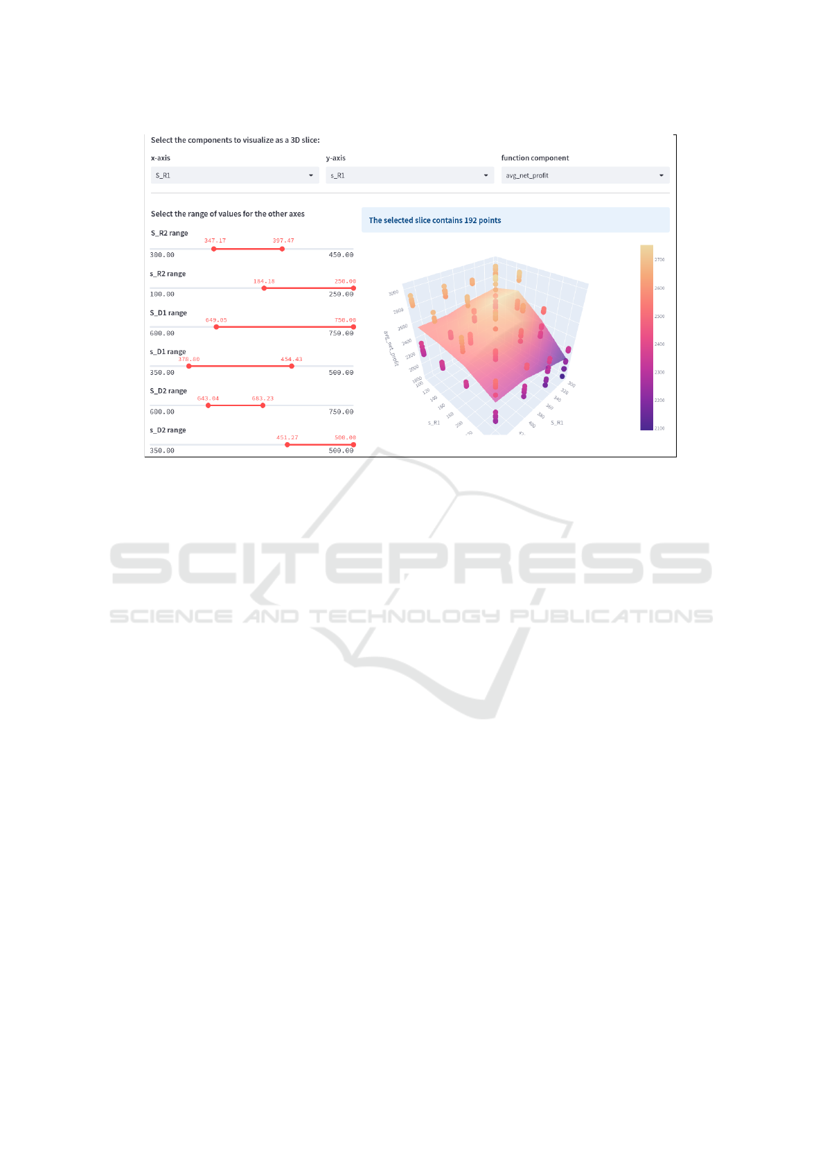
Figure 3: The DATAvis tool allows a user to visualize multi-dimensional data as 3D slices by selecting two axes at a time

and varying the values of other axes (at which the slice is taken) via interactive sliders. The GUI interface supports zoom-

ing/rotating the plot.

4.3 Meta-Model Based Optimization

The next steps in our case study are to perform opti-

mization and arrive at a general approach and design

choices for InventOpt. These choices are with regards

to the meta-model type, the number of data points

needed for building a reasonably accurate meta-model

and the choice of optimizer. To perform this explo-

ration, we ﬁrst ﬁnd optimal points in the design space

via a near-exhaustive evaluation approach. From the

set of 4

data points, we select good regions in the

design space, and perform ﬁne-grained sampling in

its neighbourhood, comparing the objective values at

each point to arrive at a point X

′

which we consider as

a reference solution. We use this as a means of eval-

uating the performance of the meta-model based ap-

proach with varying choices for the meta-model and

optimizer pairs. A meta-model g(X) provides an ap-

proximation to the original objective function f (X ),

but allows signiﬁcantly faster evaluation.

We build NN and GPR meta-models for this case

study and compare the results generated using each of

them. The meta-model parameters were tuned sepa-

rately. Out of the 4

points, we select random sub-

sets consisting of 25%, 50% and 75% points as the

training data, and the remaining points as test data to

evaluate each meta-model. For each choice we re-

port the extent of the match with the test points as

a mean squared error (MSE), summarized in Table

1. Python’s scikit-learn library (Pedregosa et al.,

2011) was used for building the meta-models. The

average computational time for building a GPR meta-

model varied between 1000-7000 seconds depending

on the training set size. For a NN model, the time

for building and training the NN model varied from

300 to 1500 seconds. Once a meta-model is built,

continuous, gradient-based optimizers can be applied

over it to quickly identify promising regions in the

design space. To arrive at a choice of optimizer for

InventOpt, we consider multiple optimizers available

in Python’s SciPy library that are well-suited for this

class of problems. The optimizers are listed in Table

1. COBYLA and Powell are trust region-based op-

timization methods while SLSQP and Nelder-Mead

are gradient-based methods and are popular choices

for black-box optimization problems. We choose

to use local optimizers rather than global optimiz-

ers because the idea is to utilize gradient informa-

tion to quickly converge to regions of interest. One

can use global optimizers such as Simulated Anneal-

ing which are more suited when the objective func-

tion is erratic or lacks trends. While this case study

only considers local optimizers, we plan to incorpo-

rate a wider choice of optimizers in the InventOpt tool

in future. Since the objective function may be non-

convex we perform multiple optimization runs with

random starting points for each optimizer. Figure 4

shows the convergence trends for each of these op-

An Open Tool-Set for Simulation, Design-Space Exploration and Optimization of Supply Chains and Inventory Problems

437

Table 1: Results obtained using multiple optimizers over a GPR meta-model built using varying sizes of training data.

Training

Dataset

Size

MSE Optimizer

Optimum

Objective

Value

Avg Number

of g(X)

Evaluation

Avg Time to

Compute g(X)

(seconds)

Distance

to Reference

Solution X

′

25%

(16,385 training

points)

0.0008

COBYLA 4203.5 355 0.0239 156.5

Powell 4327.5 346 0.0297 10.0

SLSQP 4203.5 172 0.0321 156.5

Nelder-Mead 4296.1 861 0.0294 105.9

50%

(32,768 training

points)

0.0015

COBYLA 4736.3 318 0.0726 109.0

Powell 4780.6 348 0.0635 10.0

SLSQP 4736.3 149 0.0587 109.1

Nelder-Mead 4736.3 878 0.0987 109.1

75%

(49,152 training

points)

0.0037

COBYLA 4882.7 339 0.0685 157.5

Powell 5082.1 314 0.0717 10.3

SLSQP 4882.7 145 0.0775 157.5

Nelder-Mead 5082.1 869 0.0764 10.2

timizers. Each subplot shows 20 optimization runs

with distinct, randomly chosen starting points. The

plot shows how the lowest g(X) value found varies

as the number of objective evaluations increases and

presents a rough, visual estimate of the average con-

vergence time for each optimizer. We observe that

several runs in SLSQP and Powell converge faster,

though COBYLA and Nelder-Mead are resilient to

noise. We observed that for the NN model the qual-

ity of results did not improve signiﬁcantly with the

size of training data, and the GPR model yielded con-

siderably better results compared to the NN model.

This may be because of the local minima inherently

present in the NN model. The results for the GPR

model are listed in Table 1 and summarized next. The

last column in Table 1 shows the Euclidean distance

between the optimum found by an optimizer (choos-

ing the best among the 20 independent runs) and X

′

(the reference solution).

4.4 Results and Insights

Observations from the meta-model based optimiza-

tion case study show that the GPR model performs

signiﬁcantly better than the NN model in terms of the

quality of solutions found. This could be attributed

to the non-smooth approximation surface in the NN

model. We observe that the quality of results ob-

tained with the NN model do not show any signif-

icant improvement with respect to the training set

size. However the NN model was found to be about

3x to 5x faster to train/build compared to the GPR

model. A more exhaustive evaluation of NN mod-

els with other architectures needs to be performed in

future. The GPR meta-model showed improved ac-

curacy (indicated by the MSE with respect to the test

data) with increasing training data-set sizes. The re-

sults for the GPR model are summarized in Table 1.

The GPR models provide a smoother surface for opti-

mization and gradient-based optimizers such as Pow-

ell and COBYLA are found to perform well over it.

Figure 4: Convergence plots for optimizers applied on the

GPR meta-model. The range of objective values g(X) on

the y-axis for all of the plots is from -5000 to -3000.

The number of data points required for building

the meta-model grows exponentially with the num-

ber of decision variables. Also, the computational

time for ﬁtting the meta-model grows with increas-

ing training set size. We observe that the promising

regions found by the GPR meta-models built with dif-

ferent training sizes align well, indicating that an in-

cremental sampling approach to design space explo-

ration can be used. A GPR meta-model can be ini-

tially built using a small number of training samples,

optimizers could be applied over it to locate promis-

ing regions, and these regions could be explored fur-

ther using ﬁne-grained sampling, repeated in an iter-

ative manner. Across the set of optimizers explored

in this case study, we observed that the implementa-

tion of Nelder Mead in SciPy library does not accept

parameter bounds as arguments since it is primarily

intended for unconstrained optimization. This leads

to several runs producing solutions that are outside

acceptable bounds. Although there are ways to over-

SIMULTECH 2023 - 13th International Conference on Simulation and Modeling Methodologies, Technologies and Applications

438

come this by modifying the objective function to in-

troduce penalties for out-of-bound solutions, we ob-

serve that COBYLA, Powell and SLSQP methods can

accept bounds and ﬁnd good solutions. These meth-

ods also show good convergence results. We observe

that several runs of Powell and SLSQP converge to

good solutions rapidly.

In summary, this case study provides useful in-

sights for design choices in the implementation of

InventOpt and justiﬁes the use of an iterative meta-

model based approach for a similar class of problems

in supply chain design and optimization. We plan

to generalize and incorporate the steps performed in

this case study into conﬁgurable, user-guided semi-

automated routines in the InventOpt tool-set.

5 CONCLUSIONS

This paper presented the design overview and work-

in-progress status of InventOpt - a Python-based open

tool-set for simulating, analysing and optimizing sup-

ply chain systems. Several components of the tool-

set have been implemented, and illustrated via a de-

tailed case-study presented in this paper. The case

study considers a simple inventory optimization prob-

lem which is representative of a wide class of prob-

lems relevant to supply chains and serves to justify the

use of the meta-modeling based approach used by In-

ventOpt. The detailed comparison across a set of op-

timization methods and model types in our case study

also serves to guide us in making design decisions in

the implementation of InventOpt.

REFERENCES

(2020). Documentation for simpy. https://simpy.

readthedocs.io/en/latest/.

Ankenman, B., Nelson, B. L., and Staum, J. (2008).

Stochastic kriging for simulation metamodeling. In

2008 Winter simulation conference, pages 362–370.

IEEE.

AnyLogic (2022). Anylogic: Simulation modeling soft-

ware. (https://www.anylogic.com/).

Arena (2022). Arena: Discrete event simulation and au-

tomation software. (https://www.rockwellautomation.

com/en-us/products/software/arena-simulation.html).

Barton, R. R. (2020). Tutorial: Metamodeling for simula-

tion. In 2020 Winter Simulation Conference (WSC),

pages 1102–1116. IEEE.

Blank, J. and Deb, K. (2020). pymoo: Multi-objective opti-

mization in python. IEEE Access, 8:89497–89509.

Chang, T. H. (2022). Python library for parallel mul-

tiobjective simulation optimization. https://parmoo.

readthedocs.io/en/latest/index.html.

Chopra, S., Meindl, P., and Kalra, D. V. (2007). Supply

Chain Management by Pearson. Pearson Education

India.

Flexsim (2022). Flexsim. (https://www.ﬂexsim.com//).

Hypertools (2022). Hypertools: library for visualizing and

manipulating high-dimensional data in python. (https:

//hypertools.readthedocs.io/en/latest/).

IBM (2022). Ibm supply chain solutions: Python based li-

brary for supply chain analysis, modeling and simula-

tion. (https://www.ibm.com/supply-chain).

Kleijnen, J. P. (2009). Kriging metamodeling in simulation:

A review. European journal of operational research,

192(3):707–716.

miniSCOT (2022). miniscot: simulation tool for sup-

ply chain architecture and algorithms. (https://github.

com/amzn/supply-chain-simulation-environment).

Mustafee, N., Katsaliaki, K., and Taylor, S. J. E. (2021).

Distributed approaches to supply chain simulation: A

review. ACM Trans. Model. Comput. Simul., 31(4).

OptQuest (2022). Optquest: Opimisation engine. (https:

//www.opttek.com/).

Pedregosa, F., Varoquaux, G., Gramfort, A., Michel, V.,

Thirion, B., Grisel, O., Blondel, M., Prettenhofer,

P., Weiss, R., Dubourg, V., Vanderplas, J., Passos,

A., Cournapeau, D., Brucher, M., Perrot, M., and

Duchesnay, E. (2011). Scikit-learn: Machine learning

in Python. Journal of Machine Learning Research,

12:2825–2830.

Supplychainpy (2022). Supplychainpy: Python based

library for supply chain analysis, modeling and

simulation. (https://github.com/KevinFasusi/

supplychainpy).

An Open Tool-Set for Simulation, Design-Space Exploration and Optimization of Supply Chains and Inventory Problems

439