Behavioral Modeling of Real Dynamic Processes in an

Industry 4.0-Oriented Context

Dylan Molini

, Kurosh Madani and V

eronique Amarger

LISSI Laboratory EA 3956, Universit

e Paris-Est Cr

eteil, S

enart-FB Institute of Technology,

Campus de S

enart, 36-37 Rue Georges Charpak, F-77567 Lieusaint, France

Keywords:

Industry 4.0, Machine Learning, Unsupervised Clustering, Multi-Modeling, Temporal Prediction.

Abstract:

With the Industry 4.0, new fashions to think the industry emerge: the production units are now orchestrated

from some decentralized places to collaborate to improve efﬁciency, save time and resources, and reduce costs.

To that end, Artiﬁcial Intelligence is expected to help manage units, prevent disruptions, predict failures, etc.

A way to do so may consist in modeling the temporal evolution of the processes to track, predict and prevent

the future failures; such modeling can be performed using the full dataset at once, but it may be more accurate

to isolate the regions of the feature space where there is little variation in the data, then model these local

regions separately, and ﬁnally connect all of them to build the ﬁnal model of the system. This paper proposes

to identify the compact regions of the feature space with unsupervised clustering, and then to model them with

data-driven regression. The proposed methodology is tested on real industrial data, obtained in the scope of

an Industry 4.0-oriented European project, and its accuracy is compared to that achieved by a global model;

results show that local modeling achieves better accuracy, both during learning and testing stages.

1 INTRODUCTION

In the constant search for greater efﬁciency, the in-

dustrial sector has never stopped mutating; nowadays,

the Industry 4.0 proposes to rethink the way industry

is managed. To that end, hyper-connectivity and Arti-

ﬁcial Intelligence are combined to propose new fash-

ions to manage processes (Pozzi et al., 2023).

Real dynamic industrial systems are complex:

they might evolve suddenly toward unwanted direc-

tions for any reason, which may affect efﬁciency;

such events are known as disruptions, or anomalies.

They should be prevented from occurring as soon as

possible to avoid their propagation to other processes

(Latham and Giannetti, 2022). A possible way to do

so could be to use Artiﬁcial Intelligence to identify

and point out anomalies, such as by building predic-

tive models to estimate how the system will evolve.

System modeling is a common task in Machine

Learning, especially with time series such as histori-

cal data, for instance by using data-driven regressors.

However, due to the likely heterogeneity in the data,

feeding a regressor with a full nonlinear dataset at

once may decrease the accuracy of the approximation,

for real processes are rarely perfectly continuous.

https://orcid.org/0000-0002-6499-3959

Since an industrial process often evolves slowly, it

would be relevant to identify and model the different

parts of the process. Indeed, when a system is crafted,

it is designed to achieve some states, which are its

normal ways to behave: these states can be seen as

its regular behaviors, corresponding to the different

tasks it was crafted to perform; they should be greatly

representative of the processes (Molini

e et al., 2022).

With slowly evolving processes, the sensors of a

system should take lowly varying values when being

in such a regular state (that one may call a behavior).

Therefore, modeling these regular states separately,

and then linking the different models to each other in

some fashion, should be more accurate than modeling

the whole system at once, since it should be easier

for a regressor to approximate a lowly varying dataset

than a one with greatly different values.

As such, this paper proposes to evaluate the rele-

vancy of this approach, by splitting the system’s fea-

ture space into local regions with unsupervised clus-

tering, and then build local models upon each with

data-driven regression, which are then used to model

and predict the system’s evolution. Finally, the rel-

evancy of this structure is compared to the global

model obtained by learning from the whole dataset

at once, without passing by the split stage.

510

MoliniÃl’, D., Madani, K. and Amarger, V.

Behavioral Modeling of Real Dynamic Processes in an Industry 4.0-Oriented Context.

DOI: 10.5220/0012134500003541

In Proceedings of the 12th International Conference on Data Science, Technology and Applications (DATA 2023), pages 510-517

ISBN: 978-989-758-664-4; ISSN: 2184-285X

 2023 by SCITEPRESS – Science and Technology Publications, Lda. Under CC license (CC BY-NC-ND 4.0)

This paper is composed as follows: next section

is a short review of the literature dealing with sim-

ilar approaches; third, the methodology is detailed;

fourth, the proposed local-model-based methodology

is applied to real industrial data and is confronted to a

direct global model; last section concludes this paper.

2 STATE OF THE ART

In Industry 4.0, three areas of research may be distin-

guished: the hyper-connectivity of the units, the dig-

ital twin and the cognitive plant. Thus far, most of

the work related to Industry 4.0 has dealt with the two

ﬁrst topics, but greatly less with the third, and partic-

ularly automatic modeling of industrial systems.

On that topic, the works available are general, not

oriented toward Industry 4.0, or just discuss the future

beneﬁts of such approaches. For instance, (Cohen

et al., 2017) explains how hyper-connectivity coupled

with Artiﬁcial Intelligence should help improve efﬁ-

ciency, with a real use-case provided as example, but

only theoretically. Similarly, (Chukalov, 2017) dis-

cusses the beneﬁts of using a CPS for centralized con-

trol and how to integrate it within actual industry.

Maybe the closest work to the proposed one is

(Baduel et al., 2018), who discusses the notion of reg-

ular states and modes (behaviors), and proposes uni-

ﬁed deﬁnitions of these concepts, in the scope of test-

ing, simulation and validation, with a real use-case

provided as example; however, there is no true imple-

mentation of modeling of any sort.

Finally, it is worth mentioning (Thiaw, 2008), who

expands the notion of multi-model to nonlinear dy-

namic systems. The proposed concepts are applied to

model and predict the evolution of a real river ﬂow,

by building a multi-model and training it over histor-

ical values. The proposed multi-model based predic-

tor splits the feature space (composed of the system’s

sensors) into several intervals (sub-spaces) using ba-

sic and simple clustering (such as grid partitioning).

The obtained clusters are used to construct the set

of models and associated membership functions com-

posing the target multi-model. The ﬁnal prediction is

achieved by using polynomial interpolation of outputs

of constituent models. The accurate obtained results

make the proposed approach appealing for modeling

complex plants within the context of Industry 4.0.

Additionally, a few European projects dealing

with the future cognitive plant are worth being intro-

duced. The project COGNIPLANT proposes to use

the concept of the digital twin to create a virtualiza-

tion of real plants, i.e. a fully virtual model, in which

the control, management and modeling could be per-

formed to help the end-users (Ellinger et al., 2023).

Another project is INEVITABLE, which aims to im-

prove the control one has on the production chain by

extracting as much information as possible from un-

labeled sensor data, such as by using Bayesian opti-

mization (Toma

c et al., 2022).

Finally, another project which should be discussed

is HyperCOG, whose purpose is to investigate the fea-

sibility of the cognitive plant. To that end, fourteen

partners are gathered in the development of intelli-

gent, Machine Learning-based solutions, integrated

into a Cyber-Physical System (Huertos et al., 2021).

This paper and the proposed methodology belong to

that project, and propose a new fashion to model real

dynamic processes in an Industry 4.0 context.

3 METHODOLOGY

This paper proposes to evaluate the beneﬁts of local

modeling in an industrial context. To that end, the

feature space is split into pieces, and every region is

then modeled separately. The ﬁnal model is obtained

by linking the local models, which are later triggered

by some inputs to provide the corresponding outputs.

Notice that this paper aims to assess if multi-

modeling is suited for the prediction of industrial pro-

cesses in the context of Industry 4.0, not that cluster-

ing can isolate anomalies (see (Molini

e et al., 2022)).

3.1 Split of the Feature Space

Even though industrial processes evolve through time,

they are not directly dependent of time itself, since

the processes should evolve the same way when fed

with a same material. Therefore, the space where to

perform region partitioning will be the N-dimensional

feature space spanned by the N sensors of the system.

Clustering consists in gathering data sharing simi-

lar features, while also isolating such groups from one

another: the goal is to ﬁnd the best borders between

the groups so as to minimize an error function.

In order to ensure the maximal generalization

capability, the proposed methodology operates in a

blind context, assuming no prior information on the

dataset; therefore, only unsupervised clustering can

be considered, such as the K-Means (Lloyd, 1982)

or the Self-Organizing Maps (Kohonen, 1982). With

respect to the observations drawn in (Molini

e and

Madani, 2022), this study will use the Bi-Level Self-

Organizing Maps (BSOMs), for they proved to be

more accurate in the identiﬁcation of an unknown sys-

tem’s behaviors than both the SOMs and K-Means,

and are resilient to outliers and sporadic events.

Behavioral Modeling of Real Dynamic Processes in an Industry 4.0-Oriented Context

511

The BSOMs are an improvement of the SOMs,

which consists in clustering several times a dataset

and then projecting all these maps into a ﬁnal one.

The operating principle of a BSOM is depicted on

Figure 1, where every hexagon of the left grid is a full

SOM, and where a same color represents the different

nodes being part of a same region, thus behavior in the

case of industrial data. The BSOMs were crafted to

compensate the stochastic aspect of the SOMs, which

often makes the results barely reproducible: a BSOM

is still stochastic, but averaging several SOMs allows

to identify and isolate the largest groups (behaviors),

while making the results more reproducible.

3.2 Modeling of Time-Series

System modeling is one of the commonest tasks in

Machine Learning; two very widespread Machine

Learning, data-driven tools for time-series modeling

and prediction are the Multi-Layer Perceptron and the

Decision Trees. The ﬁrst may be one of the most uni-

versal approximators, but are long to build and train,

and there is always a certain risk for overlearning,

thus the proposed methodology will focus on regres-

sion by decision trees. Indeed, there are greatly sufﬁ-

cient for this study, since they can accurately approx-

imate both continuous and discontinuous sets of data,

and perform well with even sporadic events.

Decision trees are a data-driven model based on a

cascade of comparisons, leading to a certain decision,

taking the form of a label or a numerical value in case

of classiﬁcation or regression, respectively. The most

common decision trees are binary, meaning that every

stage of such comparison, called ”nodes”, can take

two directions: the comparison is either true or false.

Binary trees are simple and intuitive, but may lack of

generalization capabilities, and may have difﬁculties

in modeling nonlinear data or classes.

Even though several algorithms to train decision

trees exist, they all work in much the same way: they

aim to optimize some quantities or criteria, such as the

minimization of the explained variance. This study

will use the CART algorithm (Pedregosa et al., 2011).

3.3 Combination of the Local Models

Once the local models are built upon every identiﬁed

region of the feature space, a way to select the correct

model according to the input data is needed.

A possibility to do so could be to activate several

models at the same time, and provide a weighted com-

bination of them. However, this paper only aims to

provide clues on the relevancy of local modeling in an

industrial context. For that reason, to select the cor-

Two-Level Self-Organizing Map

SOM

Database

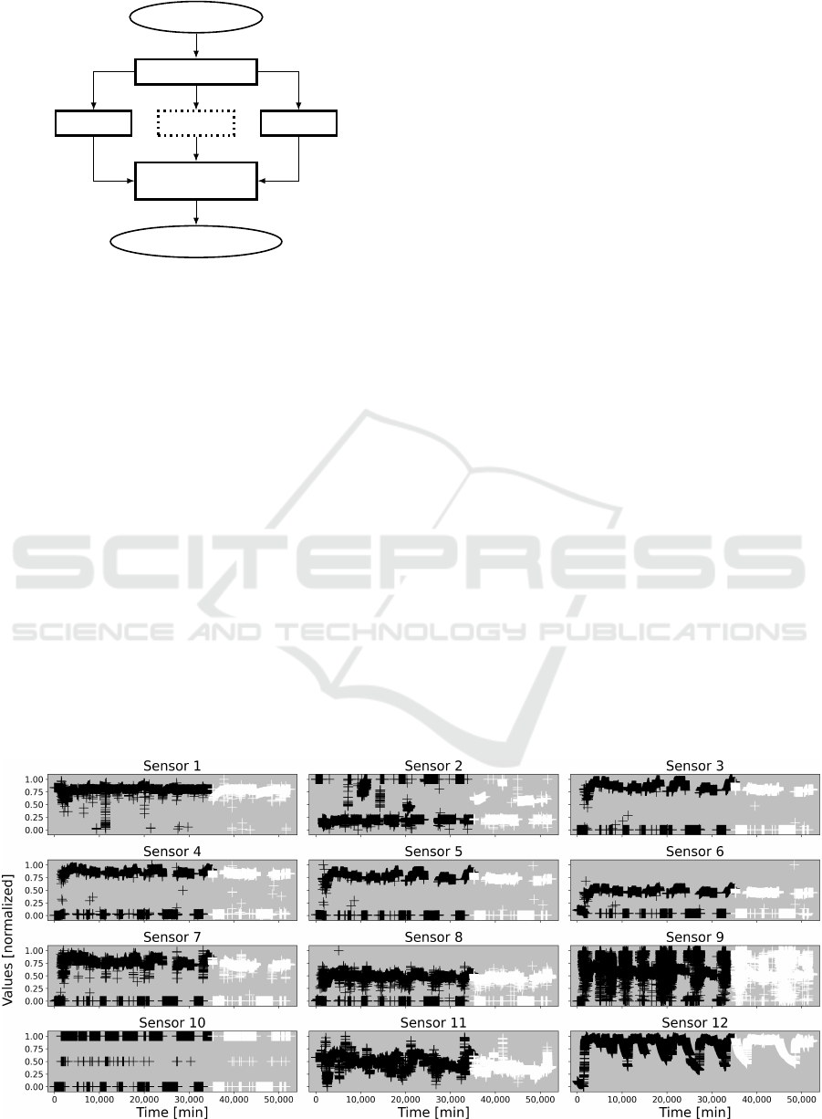
Figure 1: BSOM operating principle (picture taken from

(Molini

e and Madani, 2022)).

rect model to activate, one can compare the input vec-

tor to the behaviors’ representatives (the feature vec-

tors issued by clustering), and then trigger the model

whose representative is the closest to the input vector.

As a consequence, to select the correct model to

be activated by a given data, its distance to every clus-

ters’ barycenters must be computed, and the smallest

value indicates the closest representative feature vec-

tor, hence the correct model to activate and to use for

modeling and/or prediction. The operating principle

of the proposed methodology is depicted on Figure 2.

3.4 Quantiﬁcation of the Error

In order to evaluate the correctness of the estimates,

they should be compared to the real objective values.

To that purpose, one may consider using the Mean

Squared Error (MSE); it is deﬁned as the sum of the

squared differences between the expected outputs and

their respective estimates, normalized by the number

of values, as expressed by (1).

MSE

|D|

∑

i=1



− ˆy



(1)

where N = |D| is the cardinal of dataset D, with

D = {y

}

i∈[[1,N]]

the set of the objective values, and

{ ˆy

}

i∈[[1,N]]

is the set of the corresponding estimates.

Regarding the local models, the MSE will be com-

puted for every of them, and the total error will be

expressed as the sum of all these values respectively

weighted by their number of estimates, ﬁnally divided

by the total number of estimates, as given by (2).

MSE

|D|

∑

k=1

| × MSE

(2)

with {C

}

k∈[[1,K]]

the K clusters, such as D = ∪

k=1

Notice this measure should be interpreted rela-

tively, by comparing values to each other, since its

absolute values have no true meaning by themselves.

DATA 2023 - 12th International Conference on Data Science, Technology and Applications

512

Database

Split the database

·· ·

Model 1 Model K

Trigger the

nearest model

Global Model

Figure 2: Representation of the proposed methodology.

3.5 Materials

As mentioned in section 2, this paper is supported by

the European project HyperCOG. One of the indus-

trialists involved in the project is Solvay, a chemical

plant specialized in the production of Rare Earth spe-

cialty products. They provided the authors with a six-

month long record of a set of twelve key sensors, at

a frequency of one sample every ﬁve minutes, for a

total of 52,560 samples. Therefore, the feature space

where the proposed methodology will be applied is

that spanned by these twelve key sensors. Notice that

the Solvay’s plant has a weekly schedule: it is turned

on on Monday, and turned off on Friday, thus a motif

repeats over time; such a periodic motif helps identify

the real behaviors of the plant, and generally improves

the relevancy of the clusters issued by a BSOM. No-

tice that the sensors record different dimensions (e.g.

temperature, pressure), but normalization removes the

dimensions; as a Data-Mining approach, all sensors

are used, without distinction of their respective types.

The dataset is split into two parts, one for train-

ing, and the second for validation. Since there are

six months, a two-thirds split seems appropriate: four

months for training and two months for testing. No-

tice that successive data are used to build the subsets.

The dataset is depicted on Figure 3, where every

of the twelve sensors is represented against time. For

conﬁdentiality concerns, data have been randomized:

sensors’ tags and dimensions are removed, and values

are normalized from 0.0 to 1.0, for every dimension.

On the ﬁgure, the training and testing data are repre-

sented as black and white crosses, respectively.

4 RESULTS

To evaluate the beneﬁts of a local model-based ap-

proach compared to a direct global model, the mod-

eling will be performed in a predictive fashion, i.e.

by linking the expected outputs to the past inputs, as

expressed by ˆy

= f (x

i−µ

), with µ the prediction step.

Indeed, modeling a process itself should be highly ac-

curate, therefore the MSE would be very low for both

local and global approaches; prediction is more com-

plex, hence the MSE should be higher: the beneﬁts of

local modeling over global modeling should be eas-

ier to notice. For that reason, the step µ is set to 12,

corresponding to a prediction of an hour ahead with a

sampling rate of one value every 5 minutes.

Notice that the entire study will use all the twelve

sensors introduced in Figure 3, but only Sensors 3,

9 and 12 will be represented since they greatly differ

from one another, and the differences between the two

approaches are more easily noticeable on them.

Figure 3: The Solvay sensors’ values against time. Training and testing data in black and white, respectively.

Behavioral Modeling of Real Dynamic Processes in an Industry 4.0-Oriented Context

513

4.1 Feature Space Partitioning

The ﬁrst step of the proposed approach is to split the

feature space; to that end, a BSOM consisting of 10

SOMs of size 3 × 3 is applied to the dataset. Indeed,

with real industrial systems, one may observe a few

distinct states: the shutdown and running states, the

power on and off procedures, the transient phases,

plus some sporadic events. Therefore, one may expect

up to a ten of states at most, hence the 3 × 3 SOMs.

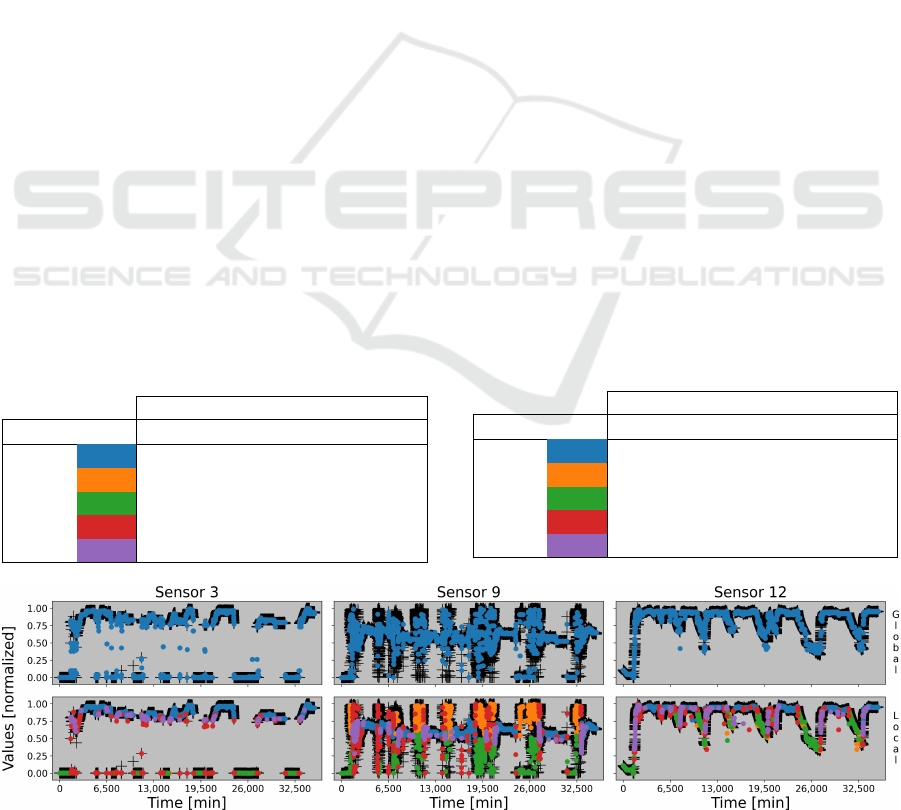
The clusters issued by the BSOM are depicted on

Figure 4, where every color corresponds to a unique

group; the color scheme and the size of the clus-

ters are summarized in Table 1. Notice that the map

comprised nine actual groups, but the smallest groups

(comprising a few data) were merged with the largest

ones for simplicity, resulting in a total of ﬁve groups.

These ones are actually representative of the regions

of the feature space, themselves representative of the

regular behaviors of the system: blue cluster corre-

sponds to the steady state, green and red ones are the

power off and on procedures, respectively, the data in

orange represent some transient state, and the purple

ones are more sporadic data, corresponding to some

transient values reached due to the processes’ inertia.

The results meet the expectations: with no prior

information, a BSOM proved able to automatically,

blindly identify the regular behaviors of a real system.

4.2 Training Local and Global Models

The second step of the proposed methodology con-

sists in building local models upon every of the behav-

iors identiﬁed in the ﬁrst stage. To that purpose, re-

gression by decision tree is used; the depth of the trees

is set to 10 in order to store as many as 2

= 1024

cases, which is expected to be sufﬁcient to represent

the about 35,000 values of the training dataset, since

there should be little variation in the data of a given

region of the feature space (the regular states).

Notice that a higher value for the depth could im-

prove accuracy, but there might be an overlearning,

thus the accuracy of the testing data would drop. For

Table 1: Color scheme and size of the clusters.

Cluster clt1 clt2 clt3 clt4 clt5

Color

Size 20,219 5709 5335 2395 1544

that reason, with respect to the size of the dataset, a

depth of 10 appears to be a good trade-off.

Figure 5 depicts the models issued when training

a decision tree with the training dataset using a global

approach (upper row) and a local one (lower row). As

a remainder, global approach means that every data

was used at the same time to build one unique model;

local approach means that every cluster got its model,

trained using only its own data. On the ﬁgure, the

objective data are represented as black crosses, whilst

the estimates outputted by the trees are represented as

colored dots (in blue for the global model, and in the

same color as the clusters for the local models, with

respect to Table 1). Notice that only the training data

and their estimates are represented on these graphs.

One may notice that global modeling tends to gen-

erate outliers, such as data whose value is around 0.4

for Sensor 3, but they are fewer with local modeling.

This is due to the sudden changes of values in data:

since there are some representatives of such values

nonetheless, the global model learnt them and returns

them when the input corresponds to a similar case,

e.g. at the junctions of differing states (behaviors).

On the opposite, with local modeling, since the differ-

ent states of the system are modeled separately, such

intermediate steps can not occur, whence the slightly

better accuracy in the estimation in that last case.

Additionally, the corresponding MSEs are gath-

ered within Table 2, for both global and local models;

in the last case, the errors of every cluster is provided.

A noticeable fact is that the errors of estimation for

Sensor 3 are always lower with every local model,

compared to that of the global model. However, lo-

cal modeling may also tend to increase the error: clt4

(red) got higher MSEs for Sensors 9 and 12; this is

due to the greater dispersion of that cluster, which is

minimized with the global model since there are al-

ways intermediate data between sudden changes. In-

Figure 4: The clusters issued by the 3 × 3 BSOM; every color corresponds to a unique cluster.

DATA 2023 - 12th International Conference on Data Science, Technology and Applications

514

deed, since red cluster contains data which do not

always follow each other, the estimation is abrupt,

whilst it is less when dealing with all data at once.

Nonetheless, the errors are smaller for the four other

clusters compared to that obtained with the global

model. Therefore, in the learning stage, local model-

ing provided more accurate estimates than global one.

4.3 Testing Local and Global Models

Now that the models are built, their accuracy must be

assessed over unknown data as of the testing dataset.

Alike the previous section, Figure 6 depicts the

original data and their corresponding estimates using

the global model (upper row) and the local models

(lower row). On the graphs, the objective data are

anew represented as white crosses, whilst the esti-

mates are colored dots (blue for the global model on

the upper row, and using the same color scheme as

Table 1 for the local models on the lower row).

First, for both approaches, the accuracy of the es-

timation is smaller than that achieved in the training

stage; this is not surprising, since the new data are ac-

tually similar, but not exactly the same, thus the corre-

sponding outputs are also similar, but not exactly the

same neither, whence the slight drop in accuracy.

Second, for both approaches anew, the models of

Sensors 9 and 12 are acceptable, but positively not

perfect: for instance with Sensor 12, from time 42,000

to time 48,000, the global model provides an almost

constant estimate, whilst there is a real decrease in

values. This also happens with the local models, but

their estimates are nevertheless closer to the objective

Table 2: The training errors of local and global models.

Sensor 3 Sensor 9 Sensor 12

Global (×10

) 1.909 5.489 0.456

Local

(×10

)

clt1 0.018 0.054 0.026

clt2 0.000 2.420 0.205

clt3 0.000 1.489 0.180

clt4 0.114 7.629 1.460

clt5 0.017 0.204 0.240

data. This limitation is directly due to the depth of

the trees: data are dropping in values, but there are

not enough leaves to store all possibilities, hence the

almost constant outputted estimates.

Third, local models issued more outliers than the

global model, fact which is noticeable with Sensor 3,

especially the red cluster (ct4). This is due to a weak

classiﬁcation of some data; indeed, it can happen that

a data is close to several clusters’ barycenters at the

same time, but only the closest is actually activated

with the actual version of the proposed methodology.

For instance, consider the case where a data would be

distant of 1 unit from a cluster, of 1.01 units from an-

other cluster, and of more than 3 units from the others;

in that case, the models of the two ﬁrst clusters should

be activated, and their respective estimates should be

fused in some fashion, since 1 and 1.01 are very close

on this scale. This is exactly what happens there:

some data are close to several clusters’ barycenters at

the same time, but only one model is activated, which

may not be the most appropriate one.

Finally, the MSEs of the predictions are gathered

in Table 3. These values emphasize the observations

made in the previous paragraph. Indeed, clt1 (blue)

got smaller MSEs than the global model, for every of

the sensors considered, since it is the largest cluster,

thus an error of classiﬁcation has a very little impact

(it is drowned out); on the contrary, clt4 (red) is it-

self rather small, thus an error of classiﬁcation has

a signiﬁcantly bad impact (wrong model activated),

whence its poor accuracy. That being said, except for

Sensor 9 and clt4, the MSEs are often smaller with

the local models compared to that of the global one.

Table 3: The testing errors of local and global models.

Sensor 3 Sensor 9 Sensor 12

Global (×10

) 12.244 23.949 5.107

Local

(×10

)

clt1 3.611 1.526 0.656

clt2 4.622 27.283 5.614

clt3 8.065 76.445 12.145

clt4 72.084 33.644 14.172

clt5 1.609 3.946 6.511

Figure 5: The global (upper) and local (lower) models trained over the training dataset.

Behavioral Modeling of Real Dynamic Processes in an Industry 4.0-Oriented Context

515

These remarks mean that a local-model-based ap-

proach works well with large behaviors, but the accu-

racy of the more sporadic events is badly affected, due

to a wrong classiﬁcation and activation of the models.

Nonetheless, with respect to the amount of estimates

of every cluster, the overall MSE is smaller when con-

sidering the local models, as shown thereafter.

4.4 Comparison for the Twelve Sensors

Thus far, the study has focused on three sensors, in

order to underpin the beneﬁts of using local modeling

on real dynamic industrial processes; nonetheless, the

nine other sensors should also be checked.

To that end, Table 4 regroups the MSEs obtained

with both approaches, for every of the twelve sensors.

For every of them, the ratio between the MSE of the

global model and that of the local models is also pro-

vided so as to ease the interpretation; indeed, if the

ratio is higher than 1, it means that global modeling

has a higher error, and the other way around if lower.

The local MSEs obtained over the training dataset

are always lower than that of the global model (all

ratios higher than 1), meaning the learning dataset has

been more accurately approximated by local models.

Consequently, one can conﬁdently state that a local-

model-based approach is beneﬁcial in order to both

model and predict (twelve steps ahead) real industrial

dynamic processes, at least when learning them.

That observation is a little more mitigated for the

testing dataset, for which, in the average, the MSEs

achieved by the local models are very often smaller

than that of the global model, except for Sensors 1

and 11. The mean of the twelve ratios is 1.744, mean-

ing that local modeling is globally beneﬁcial, for it

has decreased the error by 74%; however, it was at the

cost of a loss in accuracy for two sensors. This loss in

accuracy is due to the presence of more outliers com-

pared to the global predictor, due to the higher disper-

sion of the data of some clusters of these sensors.

5 CONCLUSION

This paper discussed the beneﬁts of using a local-

model-based approach in the scope of modeling and

predicting real Industry 4.0-related processes.

The proposed methodology consists of three steps:

ﬁrst, the system’s feature space is split by unsuper-

vised clustering, second the different regions identi-

ﬁed are modeled separately, and third the models are

eventually activated with respect to the closeness of

input data. By using a high-level averaging clustering

algorithm, the ﬁrst step aims to automatically iden-

tify and isolate the behaviors historically encountered

of any unknown system; then local modeling aims

to build a set of models to represent these behaviors.

The ﬁnal model can therefore be seen as a smart, self-

organizing combination of the system’s behaviors.

Applied to real industrial data, provided by a

real chemical plant in the scope of the Industry

4.0-orientated European project HyperCOG, this ap-

proach proved to be more accurate than directly feed-

ing the time-series into some modeling tools. That be-

havioral approach has the advantage of being simple,

not case-dependent, and requires no prior knowledge

to perform; moreover, it increases the accuracy of the

results, and diminishes the severity of the outliers.

Nonetheless, it seems that the actual way to ac-

tivate the different local models is too limited, since

it does not take into account the case when a data is

close to several clusters at the same time, and that sev-

eral models may be considered. Nonetheless, the ini-

tial objective of the paper has been achieved, i.e. as-

sessing that local modeling is an appropriate fashion

to model industrial, nonlinear dynamic processes.

Solving that limit will constitute our next work,

i.e. thinking, implementing and assessing a fashion to

intelligently activate several local models in parallel

so as to account for the possible closeness of a data to

several clusters at the same time. This fusion should

be experience-based and data-driven, therefore we are

thinking about Machine Learning optimization tools

to deal with that task, such as, why not, fuzzy logic.

Figure 6: The testing dataset’s estimates issued by the global (upper) and local (lower) models.

DATA 2023 - 12th International Conference on Data Science, Technology and Applications

516

Table 4: The training and testing errors of both local and global approaches.

Training Testing

Local

(×10

)

Global

(×10

)

Global

Local

(×10

)

Global

(×10

)

Global

Local

Sensor 1 0.039 0.220 5.687 3.146 2.377 0.756

Sensor 2 0.183 0.881 4.823 16.258 29.986 1.844

Sensor 3 0.019 1.909 99.848 4.597 12.244 2.664

Sensor 4 0.032 1.975 61.958 4.820 12.778 2.651

Sensor 5 0.330 1.173 3.556 2.602 3.935 1.512

Sensor 6 0.081 0.471 5.786 1.133 1.637 1.445

Sensor 7 0.156 1.719 11.036 3.718 9.871 2.655

Sensor 8 0.624 2.869 4.599 9.109 10.551 1.158

Sensor 9 1.175 5.489 4.672 16.546 23.949 1.447

Sensor 10 0.255 2.725 10.697 8.445 24.097 2.853

Sensor 11 0.283 0.845 2.988 3.915 1.841 0.470

Sensor 12 0.185 0.456 2.465 3.483 5.107 1.466

Mean 0.280 1.728 18.176 6.481 11.531 1.744

Standard deviation 0.314 1.409 29.212 4.933 9.278 0.763

ACKNOWLEDGEMENTS

This paper has received funding from the European

Union’s Horizon 2020 research and innovation pro-

gram under grant agreement No 869886 (project Hy-

perCOG). Authors would thank Solvay and especially

Mr. Marc Legros for their fruitful discussions.

REFERENCES

Baduel, R., Bruel, J.-M., Ober, I., and Doba, E. (2018).

Deﬁnition of states and modes as general concepts for

system design and validation. In 12e Conference In-

ternationale de Modelisation, Optimisation et Simu-

lation (MOSIM 2018), pages 189–196, Toulouse, FR.

Open Archives HAL. Proceedings published in HAL:

https://hal.archives-ouvertes.fr/hal-01989427/.

Chukalov, K. (2017). Horizontal and vertical integration, as

a requirement for cyber-physical systems in the con-

text of industry 4.0. International Scientiﬁc Journals

of Scientiﬁc Technical Union of Mechanical Engineer-

ing ”Industry 4.0”, 2(4):155–157.

Cohen, Y., Faccio, M., Galizia, F. G., Mora, C., and Pilati,

F. (2017). Assembly system conﬁguration through in-

dustry 4.0 principles: the expected change in the ac-

tual paradigms. IFAC-PapersOnLine, 50(1):14958–

14963. 20th IFAC World Congress.

Ellinger, J., Beck, L., Benker, M., Hartl, R., and Zaeh, M. F.

(2023). Automation of experimental modal analysis

using bayesian optimization. Applied Sciences, 13(2).

Huertos, F. J., Masenlle, M., Chicote, B., and Ayuso, M.

(2021). Hyperconnected architecture for high cog-

nitive production plants. Procedia CIRP, 104:1692–

1697. 54th CIRP CMS 2021 - Towards Digitalized

Manufacturing 4.0.

Kohonen, T. (1982). Self-organized formation of topolog-

ically correct feature maps. Biological Cybernetics,

43(1):59–69.

Latham, S. and Giannetti, C. (2022). Root cause classiﬁca-

tion of temperature-related failure modes in a hot strip

mill. In Proceedings of the 3rd International Con-

ference on Innovative Intelligent Industrial Produc-

tion and Logistics - IN4PL,, pages 36–45. INSTICC,

SciTePress.

Lloyd, S. P. (1982). Least squares quantization in pcm.

IEEE Trans. Inf. Theory, 28:129–136.

Molini

e, D. and Madani, K. (2022). Bsom: A two-

level clustering method based on the efﬁcient self-

organizing maps. In 2022 International Conference on

Control, Automation and Diagnosis (ICCAD), pages

1–6.

Molini

e, D., Madani, K., and Amarger, V. (2022). Cluster-

ing at the disposal of industry 4.0: Automatic extrac-

tion of plant behaviors. Sensors, 22(8).

Pedregosa, F., Varoquaux, G., Gramfort, A., Michel, V.,

Thirion, B., Grisel, O., Blondel, M., Prettenhofer,

P., Weiss, R., Dubourg, V., Vanderplas, J., Passos,

A., Cournapeau, D., Brucher, M., Perrot, M., and

Duchesnay, E. (2011). Scikit-learn: Machine learning

in Python. Journal of Machine Learning Research,

12:2825–2830.

Pozzi, R., Rossi, T., and Secchi, R. (2023). Industry 4.0

technologies: critical success factors for implementa-

tion and improvements in manufacturing companies.

Production Planning & Control, 34(2):139–158.

Thiaw, L. (2008). Identiﬁcation of non linear dynamical

system by neural networks and multiple models. PhD

thesis, University Paris-Est XII, France. (in French).

Toma

c, S., Andonovski, G.,

Skrjanc, I., and Logar, V.

(2022). Data-driven modelling and optimization of

energy consumption in eaf. Metals, 12(5).

Behavioral Modeling of Real Dynamic Processes in an Industry 4.0-Oriented Context

517