Impact of Inventory Management Policies on Supply Chain

Resilience at RiRiShun Logistics

Edward Meredith, Nikolaos Papakostas

and Vincent Hargaden

Laboratory for Advanced Manufacturing Simulation & Robotics (LAMS), School of Mechanical & Materials Engineering,

University College Dublin, D04 V1W8, Ireland

Keywords: Supply Chain Risk & Resilience, Simulation Modelling, Inventory Management, RiRiShun Logistics.

Abstract: Using one year's transaction level data from a large logistics service provider, this paper employs discrete

event simulation to assess various inventory policies for managing supply chain risks and developing

resilience. Datasets from a large Chinese Business-To-Consumer firm (RiRiShun Logistics) specialising in

the order fulfilment of household appliances were provided. Using the datasets, a discrete event simulation

model of RiRiShun's distribution supply chain in two customer regions was developed using anyLogistix

™

simulation software. A series of experiments were carried out to analyse the impact of inventory management

policies on the performance of its supply chain in the face of disruptions. Results showed that decentralised

inventory performed better when dealing with disruptions, while centralised inventory performed better when

dealing with demand uncertainty.

LIST OF ABBREVIATIONS

Table 1: List of abbreviations.

ALX an

istix™

B2B Business To Business

B2C Business To Consume

CDC Central Distribution Centre

CSV Comma-Se

arated Values

DC Distribution Centre

DES Discrete Event Simulation

LMH Last Mile Hub

LTC Local Transfer Centre

RDC Regional Distribution Centre

SKU Stock Kee

Unit

TTR Time to Recove

TTS Time To Survive

1 INTRODUCTION

Modern supply chains are highly complex, with those

firms engaged in the supply and distribution of

business to consumer (B2C) products tending to have

multi-echelon networks, often with centrally located,

https://orcid.org/0000-0002-0443-221X

https://orcid.org/0000-0003-1247-613X

larger warehouses outside urban districts and then

smaller order fulfilment facilities located closer to

clusters of customers. Such multi-echelon

distribution networks present supply chain design and

management challenges, where inventory location,

product availability and speed of order fulfilment to

end customers are key issues. Firms must manage the

trade-off between holding inventory at large upstream

warehouses, the transportation cost and order cycle

time to end customers. In the wake of the COVID-19

pandemic, there is additional focus on designing

resilient supply chains, with one approach being to

hold increased safety stock, but which comes with

increased inventory costs.

This paper employs simulation modelling and

uses transaction level data from a large B2C firm

(RiRiShun Logistics) to analyse the resilience of its

downstream distribution network, with particular

focus on the role of inventory management policies.

The analysis focuses on where best to store inventory

to lower network costs while maintaining service

levels to customers when the network is subject to

disruptions and increasing levels of demand variation.

Previous research (e.g. Berman et al., 2011) shows

that storing inventory at higher echelons mitigates

Meredith, E., Papakostas, N. and Hargaden, V.

Impact of Inventory Management Policies on Supply Chain Resilience at RiRiShun Logistics.

DOI: 10.5220/0012146800003546

In Proceedings of the 13th International Conference on Simulation and Modeling Methodologies, Technologies and Applications (SIMULTECH 2023), pages 159-168

ISBN: 978-989-758-668-2; ISSN: 2184-2841

 2023 by SCITEPRESS – Science and Technology Publications, Lda. Under CC license (CC BY-NC-ND 4.0)

159

against downstream disruptions such as stochastic

demand, while storing inventory at lower echelons

better protects against supply uncertainty.

The remainder of this paper is structured as

follows. Section 2 summarises the findings from the

relevant literature. A description and preliminary

analysis of the datasets provided by RiRiShun

Logistics is provided in Section 3. Section 4 describes

the development of the simulation model and the

experiments that are carried out. Results from the

experiments and a discussion are in Section 5.

Conclusions, limitations and future work are outlined

in Section 6.

2 LITERATURE REVIEW

This section provides a summary of the relevant

literature related to inventory management policies,

with particular focus on supply chain risk, as well as

the analytical approach employed in the paper

(Discrete Event Simulation).

2.1 Inventory Management & Supply

Chain Risk

Previous research focusing on the minimisation of

inventory costs includes Üster et al. (2008), which

identifies four dominant pillars of inventory costs:

stock-out, holding, transportation and opportunity

costs. While Üster et al. (2008) focus on minimizing

system-wide transportation costs, the research

described in our paper focuses on the role of

inventory allocation policies within a pre-existing

distribution network to enhance resilience. Initial

allocation of inventory is crucial and several methods

for initial allocation are discussed in Liu (2016) and

Catalán et al. (2012). Liu (2016) utilises the same data

set as our paper and explores the impact inventory

allocation has on transhipment and replenishment

policies. The distance between distribution centres

was identified as a crucial factor in the success of

inventory policies and in lowering overall logistics

costs. Catalán et al. (2012) explore how best to

categorise Stock Keeping Units (SKU) so those often

sold together are located at similar locations. The

allocation of SKUs in different echelons is also

discussed in Nozick & Turnquist (2001), Mao et al.

(2019) and Li et al. (2021). The first two of these

explain that less popular SKUs should be stored at a

higher echelon. There, they will accumulate lower

holding costs. This negates the additional cost they

incur when they are ordered. These papers also

emphasise the need to study the lower echelons of

supply chain networks as their inventories are more

critical to the network's profitability. Li et al. (2021)

focus on the most popular SKU from the most popular

client, an approach which significantly decreases the

complexity of the real-world problem.

Risk-pooling is a common inventory management

tactic in the context of supply chain risk management.

Risk pooling means concentrating stock in centralised

locations, while risk diversification in this context

means spreading inventory across multiple

distribution centres (DCs) to lower the impact of

disruptions.

Supply chain resilience refers to "the ability of a

system to bounce back from a setback" (Schmitt &

Singh, 2012). The necessity for a closer examination

of supply chain resilience has intensified since the

COVID-19 pandemic (Ivanov & Dolgui, 2022).

Firms no longer see disruptions as exceptional events

but rather as part of ongoing business planning,

leading to increased focus on designing resilient

supply chains.

Schmitt & Singh (2012) discuss the outcomes of

holding inventory higher or lower in the supply chain.

If a disruption occurs and the majority of inventory is

held upstream, the downstream DC's inventory will

deplete and will not be easily replenishable.

Alternatively, if a disruption occurs when inventory

is held further downstream, upstream production

output will have to be reduced unless alternative

storage facilities are available. Schmitt et al. (2015)

investigate the applicability of risk pooling and risk

diversification depending on the stochasticity of both

demand and supply. It is generally accepted that

under deterministic supply and stochastic demand, a

centralised inventory is preferred as the demand

variance of each demand can be pooled together,

lowering operational costs. Conversely, if supply is

stochastic and demand is deterministic, a less

centralised approach is favourable as disruptions will

impact the entire system less. Berman et al. (2011)

found that holding inventory centrally was beneficial

when stochasticity was introduced to a supply chain.

This research found that low variations in demand

favoured the centralised method by allowing it to

maintain adequate service levels at higher levels of

variation. At 50% variation, however, the benefits of

risk pooling ceased as the system entered a " complete

shutdown" regime. Tomlin (2006) and Park et al.

(2010) also discuss the effects of risk pooling and risk

diversification in the face of disruption, with Tomlin

(2006) arguing that risk diversification lowers

transport costs and also stating "Firms that passively

accept the risk of disruptions leave themselves open

SIMULTECH 2023 - 13th International Conference on Simulation and Modeling Methodologies, Technologies and Applications

160

to the danger of severe financial and market-share

loss".

2.2 Discrete Event Simulation

Discrete Event Simulation (DES) is a method of

modelling the operations of a system in which each

action or event that takes place changes the state of

the system and occurs at a particular time. These

times and changes are recorded within the simulation

(Law et al., 2007). DES has several advantages as an

analytical modelling approach. It enables the creation

of a complex network of interrelated operations and

the performance of various 'what-if' experiments

(Jahangirian et al., 2010). In recent years, it has been

used increasingly in supply chain management. For

instance, Haque et al. (2022) utilise DES to lower

logistics costs, Papakostas et al. (2019) to design

dynamic manufacturing networks, Liu et al. (2016) to

optimise inventory allocation and transhipment

policies and Chu et al. (2015) to sustain adequate

fulfilment rates. Furthermore, while mathematical

programming and optimisation techniques (e.g.

Linear Programming) produce a single point result,

DES provides the decision maker with a range of

results, often in the form of a distribution and

confidence interval. DES also allows for

stochasticity. The user can introduce agents

(products) into the system at a specified time or a rate

with a specified distribution. This control allows the

user to see the impact of an increased demand

variance and add a certain level of randomness,

capturing the true nature of unpredictable real-world

problems.

DES has also seen increased adoption and

application recently to model supply chain risk and

resilience. A range of studies demonstrating the

usefulness of applying this technique to disruptions

have been carried out (Ivanov, 2017; Ivanov &

Rozhkov, 2020; Ivanov & Dolgui 2022). These

studies all demonstrate how simulation allows the

user to experiment with different transportation and

stocking policies in the face of disruptions to examine

their impacts on lead times, financial outcomes and

network efficiency.

3 PRELIMINARY ANALYSIS

This section will provide an introduction to RiRiShun

Logistics (RRS) and its operations. In addition, it will

describe the transaction level data sets that were used

in this research.

3.1 Research Context: RiRiShun

Logistics

RiRiShun (RRS) Logistics is a Haier Group

subsidiary and a leading logistics service provider

focusing on home appliance delivery and installation

in China. RRS has created a distribution network that

can deal with bulkier household appliances (e.g.

cookers, refrigerators, washing machines etc.) which

require special handling and installation. In 2021,

RRS supported the Institute for Operations Research

and Management Science (INFORMS)

Manufacturing & Service Operations Management

(MSOM) Society's "Data-Driven Research

Challenge" by providing MSOM members with a

single year's actual logistics operational-level data.

The data include over 14 million orders from 149

consigners with deliveries to an estimated 4.2 million

customers in China and handles 18,000 SKUs.

The RRS distribution network is designed in a

hierarchical manner. At the top are seven national

central distribution centres (CDCs). Below are 26

regional distribution centres (RDCs); at the lowest

level there are 100 local transfer centres (LTCs).

These are serviced by more than 6,000 last-mile hubs

(LMHs), which deliver directly to the end customers.

A high level outline of the network is illustrated in

Figure 1.

Figure 1: RiRiShun Distribution Network (Guo et al.,

2021).

Typically, the logistics for each Chinese province

in RRS' service area are provided by one CDC or

RDC. However, due to the uneven population

distribution, some provinces have more than one

RDC, while others might not have any and be served

by a neighbouring province. RRS provides both

Business to Customer (B2C) and Business to

Impact of Inventory Management Policies on Supply Chain Resilience at RiRiShun Logistics

161

Business (B2B) operations, but for the focus of the

research challenge, the focus is only on its B2C

supply chain.

3.2 Data Description

RRS data consist of seven CSV files, each containing

information on a particular logistics segment. The

tables in each file describe details on individual

orders, the products being delivered, appointments

made by customers, granular delivery details, and the

customers themselves. The data sets are linked by a

standard primary key (order_no). The purpose of the

key is to provide a way to join the data from different

tables or data sets into a single table or data set. The

key matches up rows in different data sets with the

same value so that the corresponding data can be

combined into a single row. Each table also has a

foreign key to distinguish between each row of their

respective tables. Table 2 depicts the Delivery_details

data set with examples of each value.

Sometimes when a SKU is ordered, it must be

transhipped through each echelon of the distribution

network and even go through a LMH before being

delivered to a customer. Each sub-process is detailed

in the Delivery_details table. Of course, the order to

which each sub-process is a part of is detailed in the

order_no column, and the unique identifier for each

row in the table is given in the rrs_pool_node_info_id

column. When an order is placed, a DC is assigned to

track and ensure that the order is delivered. That DC

is specified through operation_center_code. As the

SKU moves closer to the customer, the warehouse

that it departs is shown in orig_code and that it enters

is dest_code. To clarify, the locations possible in the

orig_code column are origin centres, transfer centres,

destination centres and LMHs. The values possible in

the dest_code column are transfer centres, destination

centres, LMHs and the GB codes for specific Chinese

districts (Postcodes). The type of operation between

the two locations is detailed in the node_code column.

The example given in Guo et al. (2021) is "QS",

meaning "signed". This means that the orig_code and

dest_code is the name of an LMH and the customer's

location, respectively.

The Appointment_details and SKU_details tables

describe how long each order took to be delivered and

product-specific information, respectively. These

tables were merged through the order_no column to

create a table that described all transactions between

warehouses pertaining to the most frequently sold

SKU with the mean lead time of those orders. In this

way, our paper follows the methodology proposed by

Li et al. (2021) that focuses solely on the most popular

RRS SKU to reduce processing times.

3.3 Data Cleaning

To create an accurate simulation model of the RRS

network, the locations of all DCs were required.

However, RRS did not provide this information.

Instead, they provided a supplementary

Distance_information table, which contains a matrix

detailing the distances between all 103 warehouses.

Guo et al. (2021) also provided a blank map of China

depicting the locations of the CDCs and RDCs. The

locations of the LTCs were found through

triangulation. To find one LTC, circles were drawn

digitally around three known locations. The radii of

each circle were given as the distance between the

three known locations and the LTC's location. Where

these three circles intersected was determined to be

the approximate location of the LTC. Figure 2

illustrates the locations of all RRS DCs and LTCs.

The CDC icons are navy, the RDC icons are blue and

the LTC icons are green.

Figure 2: Location of RRS distribution centres.

Table 2: Description of the Delivery_details table.

Fiel

Data Type Sample Value

rrs_pool_node_info_i

igin

01a967a7bda6a071e7b4f71275e102aa

order_no varcha

0d0a09d33b1190313a392d619e9d223a

operation_center_code varcha

RRSZX076

orig_code varcha

rrs

3927

dest_code varcha

GB00264

node_code varcha

node_operation_date datetime 2019-06-04 23:59:59

SIMULTECH 2023 - 13th International Conference on Simulation and Modeling Methodologies, Technologies and Applications

162

3.4 Data Construction

To create a model that accurately represents the RRS

network, the number of times each DC sent a product

to and received a product from another DC had to be

known. Since RRS only provided the locations of

DCs and not LMHs, this paper will only focus on

interactions between the top three echelons of the

network. Consequently, the model will treat all LTCs

as customers, whereas CDCs and RDCs will be

treated as DCs. To generate the number of times each

DC sent and received a product from another DC, the

Delivery_details data set required cleaning. All rows

where the sender and the receiver of the product were

not named had DCs deleted. Moreover, the

Delivery_details documented processes that did not

involve two DCs, but rather a process that started and

finished within the same DC. Rows, where the sender

and the receiver were the same, were also deleted.

Table 3 depicts the top five rows of the data frame

created (using Python) during the data construction

phase. The data represents only the most frequently

sold SKU (1936c558) in the busiest quarter of the

year (June to August). Each combination of sender

and receiver was created and counted. This data frame

also showed that, within the top three echelons of the

network, LTCs rarely sent SKUs, while CDCs and

RDCs seldom received SKUs. This demonstrates that

modelling the first two echelons of the network as

DCs and the LTC echelon as customers is

appropriate.

Table 3: Top five rows of the “combinations count” data

frame.

Index Sende

- Receive

Count

0 RRSZX081 - RRSZX083 5,867

1 RRSZX033 - RRSZX021 4,949

2 RRSZX083 - RRSZX086 4,059

3 RRSZX043 - RRSZX048 3,802

4 RRSZX074 - RRSZX079 3,429

4 SIMULATION MODELLING

In this section, an outline of the simulation modelling

approach will be provided. Based on this, an

experimental test design will be generated, so that

different questions in relation to the impact of

inventory management policies on supply chain

resilience can be answered. Section 2 previously

discussed the appropriateness of DES to analyse

supply chains (e.g. Chu et al., 2015; Liu et al., 2016;

Papakostas et al., 2019; Haque et al., 2022 all used

this modelling approach to generate results for their

respective research). As previously mentioned, DES

has advantages over other approaches: its ability to

consider stochasticity, disruptions and real-time

monitoring of a supply network. Li et al. (2021)

asserts that DES allows an entire network to be

considered and optimised rather than one specific

aspect. The modelling software used by Li et al.

(2021) was AnyLogic. In 2014, AnyLogic created a

spin-off product to deal specifically with simulation

modelling of supply chains called anyLogistix™

(ALX). ALX allows users to create a digital twin of

supply chains of any size to design and optimise

network features and strategies. ALX has been

previously used to model disruptions and to analyse

what-if scenarios (Ivanov, 2017; Ivanov & Rozhkov,

2020; Ivanov & Dolgui 2022).

4.1 Simulation Model Development

ALX enables the creation of a simulation model to

simulate and test supply chain scenarios for RRS to

evaluate its supply chain performance, with particular

focus on inventory management policies and their

impact on supply chain resilience. The model is

designed to focus on metrics such as service levels,

lead times, inventory costs and transport distances.

The model's features include the DCs/factories,

customers, locations, demand data, suppliers and

vehicles. The locations of each DC and customer are

based on real DCs in the RRS network and are

connected automatically in the ALX model using

accurate road network data. The demand for each

customer was found by analysing the RRS data for

the busiest quarter of the year and a demand

coefficient was applied to each month based on the

number of transactions done per month. The lead time

for product 1936c558 was found to be 42 hours,

which was chosen as the expected delivery time, and

orders were dropped if delivery was not possible

within this period.

4.2 Experimental Design

ALX functionality provides a range of experiments to

run. The most basic, “Simulation Experiment”,

simply simulates the model that the user creates.

However, other experiments exist that focus on safety

stock and risk analysis. Ivanov (2017) used the basic

“Simulation Experiment” to assess the performance

of different inventory policies. When running one of

these experiments, the user can specify a start and end

date, create dashboards to show the simulation results

and when imposing demand stochasticity, specify

how many iterations of the experiment to run. The

Impact of Inventory Management Policies on Supply Chain Resilience at RiRiShun Logistics

163

user can then adjust the model, rerun the simulation

and compare the results. The experiments described

in our paper were focused on two of RRS's customer

regions in China: Foshan and Chengdu.

This research aims to answer two primary

questions regarding the impact of inventory

management policies on supply chain resilience. The

first question is whether RRS supply chain network

performs better if most of its stock is centrally held at

a higher echelon of the supply chain or if the stock is

held in decentralised locations at a lower level of the

supply chain network. While prior literature

discussed appropriate safety stock levels and

inventory policies to deal with disruptions (e.g.

Schmitt et al., 2015), it appears none to date have

investigated whether keeping stock upstream or

downstream makes supply chains more resilient. Two

important metrics of supply chain resilience are Time

To Survive (TTS) and Time To Recover (TTR)

(Simchi-Levi et al., 2014; Nguyen, 2021). TTS is the

length of time a supply chain can maintain adequate

service levels after a disruption, while TTR is the time

it takes a supply chain to achieve normal service

levels after the drop caused by the disruption.

The second research question is how stochastic

demand affects the performance of RRS supply chain

network. Prior research has shown that holding

inventory centrally can better cope with the

stochasticity of demand when supply is deterministic,

due to the risk-pooling effect where the variance of

all customers is pooled together to create one demand

variance rather than several (Schmitt et al., 2015).

However, when demand is deterministic and supply

is stochastic, a decentralised network where the

inventory is more dispersed is better suited. While

some authors have explored these findings, there has

been little examination of how networks with

centralised and decentralised stock cope with demand

variance. Although ALX software makes varying

demand easy, it is more difficult to add stochasticity

to supply. Another previous study found that a central

system could perform well at higher levels of demand

variation, but at a certain threshold, the benefits of

holding inventory centrally become negligible as the

system naturally holds no safety stock (Berman et al.,

2011).

Assumptions for each model variation are

discussed in the following sub-sections. By

configuring the model in this way, it is possible to test

different scenarios and accurately record the key

performance indicators (KPI) of the supply chain.

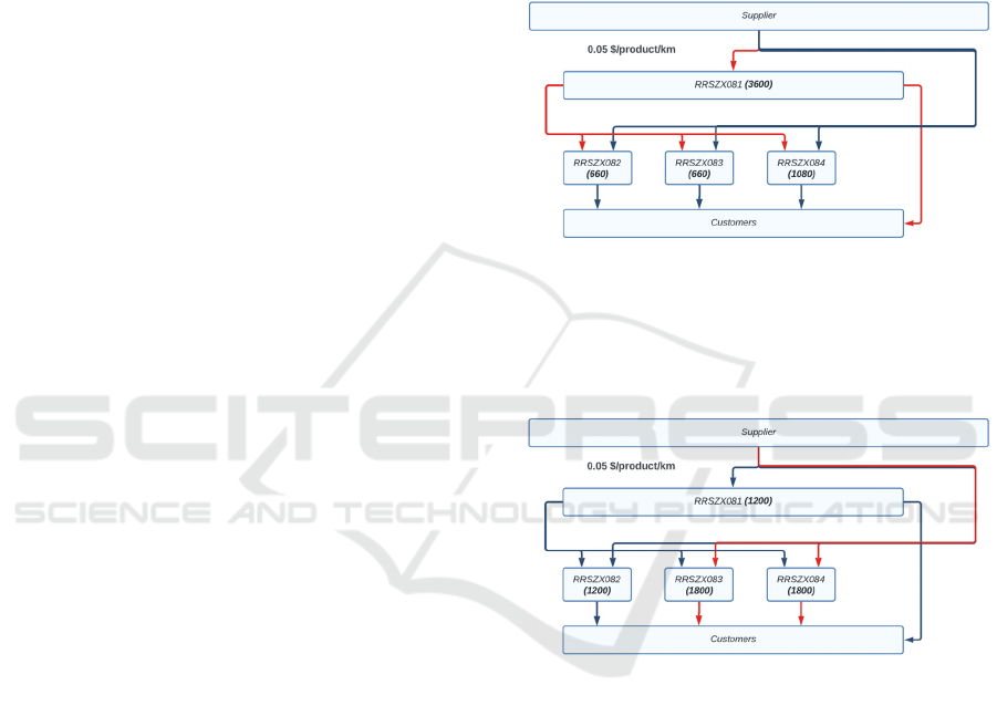
4.2.1 Upstream Versus Downstream

It was decided that the model would have a capacity

of 6,000 units. To differentiate between a centralised

and decentralised network, these 6,000 units would be

separated in different ways. For the centralised

network, 60% of the capacity was allocated to the

CDC. The remaining 40% were dispersed based on

demand. The capacities for each DC in the Upstream

model can be seen in Figure 3.

Figure 3: Product flow – upstream model.

The decentralised model more evenly dispersed

the 6,000 units. Two DCs were allocated 30% of the

6,000 units while the other two DCs were allocated

20% each (Figure 4).

Figure 4: Product flow – downstream model.

Both models only allow the products to move

downwards through the distribution network and the

LTCs act as customers. The red lines in Figures 3 and

4 indicate the impact of the disruption. The first

experiment is examining each model's reaction to a

full DC closure where no products can flow into or

out of the closed DC. The disruption will last 30 days

and, in both cases, will impact 60% of the capacity of

the network. Therefore, the CDC in the Upstream

model carrying 60% network capacity will close,

while two RDCs carrying 30% of the network

capacity will close in the Downstream model. An (r,

Q) was used for the DCs in both scenarios where r

was one-third of the DC capacity and Q was two-

thirds of the DC capacity.

SIMULTECH 2023 - 13th International Conference on Simulation and Modeling Methodologies, Technologies and Applications

164

4.2.2 Demand Variance

This experiment introduces downstream disruptions

in the form of varying the demand of each customer.

A sensitivity analysis was performed to do this. In the

Upstream and Downstream models with disruptions,

the customers were given a demand with a triangular

distribution. The former weekly demand was the

mode value. In contrast, the minimum and maximum

values were changed for each experiment since

Berman et al. (2011) found that the benefits of risk

pooling became negligible at 50%, the minimum

values were chosen to be 80%, 60%, and 40% of the

mode value. In contrast, the maximum values were

chosen to be 120%, 140%, and 160% of the mode

value. This range should indicate how demand

variation affects both models while triggering the

threshold at which the models enter the “Complete

Shutdown” regime.

5 RESULTS & DISCUSSION

This section outlines the results obtained through the

experimentation process and discusses their findings.

5.1 Upstream Versus Downstream

Before comparing how the Upstream and

Downstream models coped with 60% capacity

disruptions, the two scenarios must be compared

performing without any issues. Table 4 contains

results from the four simulations that were run for this

experiment. The first thing to note is that both models

had an almost perfect service level. The Upstream and

Downstream models dropped two and one order,

respectively, out of a total of the 210 that was

expected. In both cases, the service level remained

above 90% the entire time.

Schmitt et al. (2015) state that a network structure

that holds its inventory downstream in more

decentralised locations will be better adapted to

handle disruptions. It would appear from the

simulation results that is accurate. Upon a 60%

capacity disruption, the TTR value for the Upstream

model was 175 days compared to 91 days in the

Downstream equivalent. This suggests significantly

higher resilience. The Total Service Level of each

model reinforces this point. The mean service level of

the Upstream model fell from 99% to 91%, almost

twice as great a decrease as the Downstream model.

It can be seen in Figures 5 and 6 that the service level

of both models reaches approximately 65% by day

30. However, where the Downstream model recovers

after that, the Upstream model continues to fall

another 10% by day 45. This indicates that the

disruption impacts the Upstream model more

aggressively and enforces a longer recovery time.

Schmitt et al. (2015) argued that by "Not putting

all the firms' eggs in one basket" a supply chain would

be less affected by disruptions, "although the same

number of eggs may be destroyed, they are not all

destroyed at once". When the majority of stock is held

at one location, the other locations are worse prepared

to deal with a sudden increase in demand.

Based on the results from this experiment, it is

suggested that inventory should be held downstream

in decentralised locations if there is a risk of

disruptions. The lesser impact sustained and quicker

recovery times suggest that holding stock at

RiRiShun's RDC levels increases its supply chain's

resilience and maintains higher levels of customer

satisfaction.

Figure 5: Service level of upstream model with disruptions.

Table 4: Results from upstream and downstream simulations (with & without disruptions).

Scenario Upstream Downstream

Version No Disru

tion Disru

tion No Disru

tion Distru

tion

Distance Travelled

(

)

158,583 151,499 208,805 202,229

Dro

ed Orders 2 19 1 10

Total Service Level 0.90 0.91 0.995 0.952

Days Below 90% Service Level 0 175 0 91

Impact of Inventory Management Policies on Supply Chain Resilience at RiRiShun Logistics

165

Figure 6: Service level of downstream model with

disruptions.

5.2 Demand Variance

Berman et al. (2011) and Schmitt et al. (2015) found

that holding inventory in a central location rather than

several decentralised locations was beneficial when

the demand from multiple customers had variation.

The reason for this was based on the work done by

Chen & Lin (1989) emphasising the benefits of risk

pooling. If one DC serves multiple customers with

demand stochasticity, all variations can be combined

to mitigate risk.

According to the results in Table 5, the effects of

demand variation are handled better in the Upstream

model. The number of dropped orders decreases as

the demand stochasticity increases. This contrasts

with the Downstream model where the number of

dropped orders increases slightly. Total Service Level

is inversely proportional to the number of dropped

orders in a network which explains the increasing

service level in the Upstream model and the

decreasing service level in the Downstream model.

While the Upstream model performs better,

neither system appears to be affected significantly by

the demand variation as much as expected. The

Upstream model appears to perform better as the level

of variation increases. Berman et al. (2011) stated that

a centralised system could operate at normal levels

for more extreme variation. However, that research

also suggested a threshold at which the benefits of

risk pooling would diminish. That threshold was

found to be 50%. However, the results from this

experiment show that at 60% variation, the benefits

of risk pooling are even more evident.

One explanation for this could be how Berman et

al. (2011) define the "Complete Shutdown" regime

where holding inventory centrally no longer realises

a benefit. In that paper, the model stops holding safety

stock due to the variation in demand. As the inventory

in each DC is 0, all met demand is that which is back-

ordered. Since no back-ordering is allowed in the

ALX model, the only demand that can be met is

orders with the required stock. The CDC in the

Upstream model has a larger reserve of stock

throughout the simulation and, therefore, can handle

larger orders. As the demand fluctuates, larger orders

that high-capacity DCs can meet become more

common. Since the Downstream model spreads its

inventory more evenly across the four DCs, those

larger orders that occur at 60% variation are less

likely to be met. This can explain the higher number

of days with an inadequate mean service level in the

Downstream model.

Building on previous literature, the results of the

simulation experiments suggest that supply chains

that see large demand fluctuations would be better to

hold stock centrally. Holding stock in fewer locations

makes infrequent large orders more likely to be met.

The benefit of risk pooling was also identified in this

experiment. Supply chains that are prone to risks and

demand stochasticity require a more detailed

examination, as the results from the first two

experiments in this thesis promote two different

inventory strategies.

6 CONCLUSIONS

This section summarises the findings of the

simulation experiments based on RiRiShun data for

Table 5: Results from the demand variance experiment.

Scenario Upstream Downstream

Version Disruption +

- 20% +

- 40% +

- 60% Disruption +

- 20% +

- 40% +

- 60%

Distance

Travelled

(

)

17,080 19,186 16,575 20,838 17,993 18,152 18,244 17,994

Dropped

Orders

19 17 17 5 10 10 11 12

Total

Service

Level

0.91 0.919 0.919 0.976 0.952 0.952 0.948 0.943

SIMULTECH 2023 - 13th International Conference on Simulation and Modeling Methodologies, Technologies and Applications

166

two of its regions in China. In the scenario where

disruptions are probable or where risk analysis of its

supply chain is in the early phases, decentralised

inventory storage is preferred. This option leaves

customers with more options from which to receive

demand. Disruptions, particularly ones where DCs

close entirely, impact supply chains with inventory

held Upstream more severely and impose a longer

TTR. While decentralised networks are advantageous

for disruptions higher in the network hierarchy,

centrally held stock takes advantage of risk pooling to

mitigate the risks associated with demand variations.

This results showed that an increase in the volatility

of demand had little effect on the Upstream model

while having greater and negative impacts on the

Downstream model.

The results from the simulation experiments align

with those of Schmitt et al. (2015) in suggesting that

supply chains with decentralised inventory are better

equipped to deal with disruptions. With more non-

disrupted DCs to complete orders, there is a higher

order completion rate. However, Upstream models

are more adept at coping with demand fluctuations.

The results also agree with the work done by Berman

et al. (2011), citing risk pooling as the reason for this.

There were differences in the results of the

simulation experiments to those described by Berman

et al. (2011), who outlined the demand variance

threshold at which Upstream supply chains no longer

had an advantage over Downstream models. The

results from our experiments suggested that Upstream

models would become increasingly effective at

dealing with demand fluctuations. As the spread of

order sizes increases, there will be more orders that

large stores of inventory can only fulfil.

There were a number of limitations to the research

described in this paper. RRS provided the datasets to

the MSOM Data-Driven Research Challenge to

facilitate academic researchers to carry out a range of

analytical studies. However, no direct contact was

provided by either RRS or MSOM to aid researchers

in improving these policies or to provide valuable

context to some of the data. One aspect of the supply

chain that could have used clarification is whether

orders could be split between two DCs to meet

demand. This was highlighted as beneficial to supply

chain performance but was not implemented in the

ALX model.

Both the Upstream versus Downstream and

Demand Variance experiments focused on how

supply chains with centralised and decentralised

inventory react to disruption in the form of DC

closures and demand fluctuation. However, there was

an experiment to investigate the optimal location of

stock when both types of disruptions are introduced.

A suggestion for further research would be to

introduce a variety of disruptions and apply them in

specific combinations to see where the inventory

should be held in each of those scenarios.

Additionally, RRS provides a good framework to

experiment with different supply chain structures.

While the research described in this paper focused

initially on two of RRS regions in China, there are a

further five regions with different geographies and

structures. It would be interesting to apply disruptions

to all seven regions and examine the effects of

network geography on supply chain resilience.

Further progress in this area might lead to the

development of a framework whereby supply chain

decision makers can decide what the best national

inventory strategies are solely by examining the

structure of the supply chain network.

ACKNOWLEDGEMENTS

Access to the datasets used in this paper was provided

through the partnership between RiRiShun Logistics

(a Haier Group subsidiary) and the Institute for

Operations Research & Management Science

(INFORMS) Manufacturing & Service Operations

Management (MSOM) Society for the 2021 Data

Driven Research Challenge.

REFERENCES

Almeder, C., Preusser, M., & Hartl, R.F. (2009). Simulation

and optimization of supply chains: Alternative or

complementary approaches? OR Spectrum, 31, 95-119.

Berman, O., Krass, D., & Tajbakhsh, M.M. (2011). On the

benefits of risk pooling in inventory management,

Production and Operations Management, 20, 57-71.

Catalán, A., Fisher, M. L., Liu, J., Minyard, C., Wang, J.,

Han, J., Huang, A., & Lai, J. (2012). Assortment

allocation to distribution centers to minimize split

customer orders. Available at SSRN 2166687.

Chen, M.-S. & Lin, C.-T. (1989). Effects of centralization

on expected costs in a multi-location newsboy problem.

Journal of the Operational Research Society, 40, 597-

602.

Chu, Y., You, F., Wassick, J. M., & Agarwal, A. (2015).

Simulation-based optimization framework for multi-

echelon inventory systems under uncertainty.

Computers and Chemical Engineering, 73,1-16.

Guo, X., Yu, Y., Allon, G.,Wang, M., & Zhang, Z. (2021).

RiRiShun Logistics: Home appliance delivery data for

the 2021 Manufacturing & Service Operations

Management Data-Driven Research Challenge.

Impact of Inventory Management Policies on Supply Chain Resilience at RiRiShun Logistics

167

Manufacturing & Service Operations Management (in

press).

Haque, S., Eberhart, Z., Bansal, A., & McMillan, C. (2022).

Semantic similarity metrics for evaluating source code

summarization, IEEE Computer Society, March, 36-47.

Ivanov, D. (2017). Simulation-based ripple effect

modelling in the supply chain. International Journal of

Production Research, 55(7), 2083-2101.

Ivanov, D. & Dolgui, A. (2022). Stress testing supply

chains and creating viable ecosystems. Operations

Management Research, 15, 475–486.

Ivanov, D. & Rozhkov, M. (2020). Coordination of

production and ordering policies under capacity

disruption and product write-off risk: an analytical

study with real data-based simulations of a fast-moving

consumer goods company. Annals of Operations

Research, 291, 387-407.

Jackson, I., Tolujevs, J., & Reggelin, T. (2018). The

combination of discrete-event simulation and genetic

algorithm for solving the stochastic multi-product

inventory optimization problem. Transport and

Telecommunication, 19, 233-243.

Jahangirian, M., Eldabi, T., Naseer, A., Stergioulas, L. K.,

& Young, T. (2010). Simulation in manufacturing and

business: A review. European Journal of Operational

Research, 203(1), 1-13.

Law, A. M., Kelton, W. D., & Kelton, W. D. (2007).

Simulation modeling and analysis, McGraw-Hill, 3

edition.

Li, C., Liu, S., Qi, W., Ran, L., & Zhang, A. (2021).

Distributionally robust multilocation newsvendor at

scale: A scenario-based linear programming approach.

Available at SSRN.

Liu, H. (2016). Simulation of lateral transshipment in order

delivery under e-commerce environment. International

Journal of Simulation and Process Modelling, 11(1),

51-65.

Mao, H., Wu, T., Li, Y., & Chen, D. (2019). Assortment

selection for a frontend warehouse: A robust data-

driven approach. Proceedings of the 49th International

Conference on Computers and Industrial Engineering

56-64.

Nguyen, H., Sharkey, T. C., Wheeler, S., Mitchell, J. E., &

Wallace, W. A. (2021). Towards the development of

quantitative resilience indices for Multi-Echelon

Assembly Supply Chains. Omega, 99, 102199.

Nozick, L. K. & Turnquist, M. A. (2001). Inventory,

transportation, service quality and the location of

distribution centers. European Journal of Operational

Research, 129(2), 362-371.

Papakostas, N., Hargaden, V., Schukraft, S., & Freitag, M.

(2019). An approach to designing supply chain

networks considering the occurrence of disruptive

events. IFAC-PapersOnLine, 52(13), 1761-1766.

Park, S., Lee, T. E., & Sung, C. S. (2010). A three-level

supply chain network design model with risk-pooling

and lead times. Transportation Research Part E:

Logistics and Transportation Review, 46, 563-581.

Qu, T., Huang, T., Nie, D., Fu, Y., Ma, L., & Huang, G. Q.

(2022). Joint decisions of inventory optimization and

order allocation for omni-channel multi-echelon

distribution network. Sustainability, 14.

Schmitt, A. J. & Singh, M. (2012). A quantitative analysis

of disruption risk in a multi-echelon supply chain.

International Journal of Production Economics, 139,

22–32.

Schmitt, A. J., Sun, S. A., Snyder, L. V., & Shen, Z. J. M.

(2015). Centralization versus decentralization: Risk

pooling, risk diversification, and supply chain

disruptions. Omega, 52, 201–212.

Simchi-Levi, D., Schmidt, W., & Wei, Y. (2014). From

superstorms to factory fires: Managing unpredictable

supply chain disruptions. Harvard Business Review,

92(1-2), 96-101.

Tomlin, B. (2006). On the value of mitigation and

contingency strategies for managing supply chain

disruption risks. Management Science, 52(5), 639-657.

Zhu, S., Hu, X., Huang, K., & Yuan, Y. (2021).

Optimization of product category allocation in multiple

warehouses to minimize splitting of online supermarket

customer orders. European Journal of Operational

Research, 290, 556-571.

Üster, H., Keskin, B. B., & Çetinkaya, S. (2008). Integrated

warehouse location and inventory decisions in a three-

tier distribution system. IIE Transactions, 40, 718-732.

SIMULTECH 2023 - 13th International Conference on Simulation and Modeling Methodologies, Technologies and Applications

168