
Design of Double-Loop Trajectory Tracking Control System for
Mobile Robot
Zhongwei Ji
*
, Kang Zhao, Yan Ding and Tingrui Liu
*
College of Mechanical & Electronic Engineering, Shandong University of Science & Technology, Qingdao 266590, China
Keywords: Control System, Mobile Robot.
Abstract: A mobile robot means that it can autonomously perform real-time motion in a designated location, integrating
functions such as autonomous decision-making, path planning, information collection, and motion control.
For mobile robots used in various fields, motion control is the premise to achieve various tasks, and trajectory
tracking control is one of its main technologies. This paper mainly aims at the trajectory tracking of wheeled
mobile robots based on the kinematics model. Taking the position control subsystem as the outer loop and the
attitude control subsystem as the inner loop, a double-loop trajectory tracking system for mobile robots is
proposed, which is proved by Lyapunov stability theory. The stability of the system and the convergence of
tracking error are improved. The designed controller can effectively overcome the influence of unknown
disturbance and better realize the trajectory tracking of mobile robots. The simulation results verify the
validity and correctness of the control law.
1 INTRODUCTION
With the continuous development and progress of
science and technology, robot technology has also
developed rapidly. Robots have been widely used in
military, manufacturing, agriculture, science and
technology industries due to their high mobility, high
autonomy, and high environmental adaptability,
which is also an important symbol of human society
moving towards technological civilization (Qu, 2015).
At the same time, the robot itself integrates many
high-tech technologies, including mechanical
processing, automatic control, information fusion of
various sensors, information engineering,
programming technology, artificial intelligence and
other interdisciplinary subjects (Tan, 2013). This not
only promotes the progress of the robot itself, but also
promotes the improvement and progress of various
interdisciplinary disciplines. The rapid progress of
interdisciplinary technology has made the once
difficult technical problems solved.
A mobile robot means that it can autonomously
perform real-time motion in a designated location,
integrating functions such as autonomous decision-
making, path planning, information collection, and
motion control. For mobile robots used in various
fields, motion control is the premise to achieve
various tasks, and trajectory tracking control is one of
its main technologies (Hu, 2016). Trajectory tracking
control of mobile robots means that at a certain initial
position, the robot tracks the desired trajectory with
respect to time under the action of the controller, and
stably runs along the desired trajectory. The trajectory
tracking problem of mobile robots can generally be
divided into two types: trajectory tracking based on
kinematic model, trajectory tracking based on
kinematic model and dynamic model (Liu, 2020). For
the trajectory tracking problem of mobile robots,
scholars at home and abroad have proposed many
control methods. These trajectory tracking control
methods mainly include PID control (Feng, 2017),
inversion control (Zhao, 2020), nonlinear state
feedback control (Chang, 2015), fuzzy control Logic
control (Zheng, 2017), control based on extended
state observer (Zhang, 2019), etc. Sliding mode
control has the advantages of robustness and strong
anti-interference ability, so sliding mode control can
be used to deal with the trajectory tracking problem
of mobile robots.
Therefore, for the trajectory tracking of mobile
robots based on the kinematic model, this paper takes
the position control subsystem as the outer loop and
the attitude control subsystem as the inner loop, and
proposes a dual-loop trajectory tracking system for
mobile robots, which is proved by the Lyapunov
stability theory. System stability and tracking error
convergence. The designed controller can effectively
Ji, Z., Zhao, K., Ding, Y. and Liu, T.
Design of Double-Loop Trajectory Tracking Control System for Mobile Robot.
DOI: 10.5220/0012149900003562
In Proceedings of the 1st International Conference on Data Processing, Control and Simulation (ICDPCS 2023), pages 89-94
ISBN: 978-989-758-675-0
Copyright
c
2023 by SCITEPRESS – Science and Technology Publications, Lda. Under CC license (CC BY-NC-ND 4.0)
89
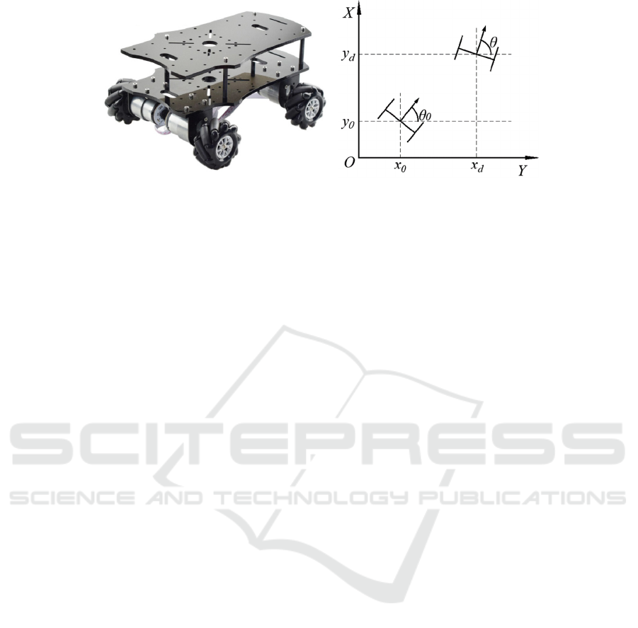
Figure 1: The mobile robot base and the schematic diagram of the motion.
overcome the influence of unknown disturbance and
better realize the trajectory tracking of mobile robots.
The simulation results verify the validity and
correctness of the control law.
2 MOBILE ROBOT KINEMATICS
MODEL
Taking wheeled mobile robots as an example, most of
these robots have two larger rear wheels, which are
driving wheels, and two smaller front wheels, which
are driven wheels. The left and right rear wheels are
each driven by a motor. If the rotational speeds of the
two motors are different, the left and right rear wheels
will generate a "differential motion", thereby enabling
cornering (Tsuchida, 2009).
A simplified model of a wheeled mobile robot
base moving in the X-Y plane is shown in Figure 1.
Define the midpoint M of the line connecting the
centers of the two driving wheels as the reference
point of the robot, then the pose P of the wheeled
mobile robot can be represented by the position
coordinates and heading angle of the reference point
M in the inertial coordinate system, where [x, y] is the
position of the mobile robot, and θ is the angle
between the forward direction of the mobile robot and
the x-axis. The control law q of a wheeled mobile
robot is represented by the linear velocity v and
angular velocity ω of the mobile robot, where v is the
position control in the control law, ω is the attitude
control in the control law, and the control input in the
kinematic model (Liu, 2020).
We might assume
𝑃
𝑥 𝑦 𝜃
(1)
𝑞
𝑣𝜔
(2)
Assuming that there is no slippage between the
wheel and the motion plane during the movement of
the wheeled mobile robot, the kinematics equation of
the wheeled mobile robot can be expressed as:
𝑝
𝑥
𝑦
𝜃
𝑐𝑜𝑠𝜃 0
𝑠𝑖𝑛𝜃 0
01
𝑞 (3)
It can be seen from the kinematics equation that
the robot model system has 2 degrees of freedom, and
the model output is 3 variables, so the model is an
underactuated system, which can only achieve active
tracking of 2 variables, and the remaining variables
are in the follow-up or steady state. This control is a
trajectory tracking problem, that is, the tracking of the
position [x, y] of the mobile robot is realized by
designing the control law, and the follow-up of the
included angle θ is realized.
From formula (3), the kinematic model of the
mobile robot can be obtained as:
𝑥𝑣𝑐𝑜𝑠
𝜃
𝑦𝑣𝑠𝑖𝑛
𝜃
𝜃
𝜔
(4)
3 TRAJECTORY TRACKING
CONTROL
Trajectory tracking control includes two parts:
position control law design and attitude control law
design. The process is to formulate a set of ideal
motion trajectories
𝑥
𝑦
𝜃
in advance, by
designing the position control law v, to realize the
actual trajectory
𝑥𝑦
tracking the ideal
trajectory
𝑥
𝑦
, and then design the attitude
control law ω to achieve the actual attitude θ tracking
the ideal attitude θ
d
. The following is the design of the
corresponding control law for the above content.
3.1 Design of Position Control Law
First, the position control law v is designed to realize
the actual position tracking the ideal position.
Define the error trajectory tracking equation as:
ICDPCS 2023 - The International Conference on Data Processing, Control and Simulation
90

𝑥
= 𝑣𝑐𝑜𝑠𝜃−𝑥
𝑦
= 𝑣𝑠𝑖𝑛𝜃−𝑦
(5)
where x
e
and y
e
represent the position error of the x-
axis direction and the y-axis direction, respectively:
𝑥
= 𝑥−𝑥
𝑦
= 𝑦−𝑦
(6)
Assume
𝑣𝑐𝑜𝑠𝜃= 𝑢
𝑣𝑠𝑖𝑛𝜃= 𝑢
(7)
For
𝑥
= 𝑣𝑐𝑜𝑠𝜃−𝑥
, take the sliding mode
function as
𝑠
= 𝑥
, then
𝑠
= 𝑥
= 𝑢
−𝑥
(8)
The design control law is
𝑢
= 𝑥
−𝑘
𝑠
(9)
where k
1
>0, so
𝑠
= −𝑘
𝑠
.
Take the Lyapunov function:
𝑉
=
𝑠
(10)
So there is
𝑉
= 𝑠
𝑠
= −𝑘
𝑠
= −2𝑘
𝑉
(11)
So that the x
e
index converges to zero.
For
𝑦
= 𝑣𝑠𝑖𝑛𝜃−𝑦
, take the sliding mode
function as
𝑠
= 𝑦
, then
𝑠
= 𝑦
= 𝑢
−𝑦
(12)
The design control law is
𝑢
= 𝑦
−𝑘
𝑠
(13)
where k
2
>0, so
𝑠
= −𝑘
𝑠
.
Take the Lyapunov function:
𝑉
=
𝑠
(14)
So there is
𝑉
= 𝑠
𝑠
= −𝑘
𝑠
= −2𝑘
𝑉
(15)
So that the y
e
index converges to zero.
From formula (7),
= 𝑡𝑎𝑛𝜃
can be obtained.
If the value range of θ is (π/2, π/2), the θ that satisfies
the ideal trajectory tracking can be obtained as
𝜃= 𝑎𝑟𝑐𝑡𝑎𝑛
(16)
θ obtained by formula (16) is the angle required
by position control law formula (9) and formula (13).
If θ is equal to θ
d
, the ideal trajectory control law
formula (9) and equation (13) can be realized, but θ
and θ
d
in the actual model equation (4) cannot be
completely consistent, especially in the initial stage of
control, which will cause the closed-loop tracking
system equation (1) unstable.
To this end, the angle θ obtained by equation (16)
needs to be regarded as an ideal value, that is, take
𝜃
= 𝑎𝑟𝑐𝑡𝑎𝑛
(17)
When designing an ideal pose instruction
𝑥
𝑦
, we must pay attention to the need to make
the value range of θ
d
satisfy (π/2, π/2).
The difference between the actual θ and θ
d
will
cause the position control laws (9) and (13) to be
unable to be accurately realized, resulting in the
instability of the closed-loop system. A simpler
solution is to make θ track θ
d
as quickly as possible by
designing an attitude control algorithm that converges
faster than the position control law.
From equation (7), the actual position control
law can be obtained as:
𝑣=
(18)
3.2 Design of Attitude Control Law
Next, the attitude control law ω is designed to make
the actual attitude θ track the ideal attitude θ
d.
For
𝜃
= 𝜃−𝜃
, take the sliding mode function
as
𝑠
= 𝜃
, then
𝑠
= 𝜃
= 𝜔−𝜃
(19)
The design control law is
𝜔= 𝜃
−𝑘
𝑠
−𝜂
𝑠𝑔𝑛𝑠
(20)
where k
3
>0, η
3
>0, so
𝑠
= −𝑘
𝑠
−𝜂
𝑠𝑔𝑛𝑠
.
Take the Lyapunov function:
𝑉
=
𝑠
(21)
So there is
𝑉
= 𝑠
𝑠
= −𝑘
𝑠
−𝜂
|
𝑠
|
≤−𝑘
𝑠
(22)
That is
𝑉
≤−2𝑘
𝑉
, so that the angle θ
exponentially converges to θ
d
.
4 THE KEY TO THE DESIGN OF
THE DOUBLE LOOP SYSTEM
The above double-loop system belongs to a closed-
loop control system composed of inner and outer
loops. The position subsystem is the outer loop, and
the attitude subsystem is the inner loop. The outer
loop generates an intermediate command signal θ
d
and
transmits it to the inner loop system. The inner loop
passes the sliding mode control law. Realize the
tracking of this intermediate command signal. The
structure of a closed-loop system with double loops is
shown in Figure 2.
Design of Double-Loop Trajectory Tracking Control System for Mobile Robot
91
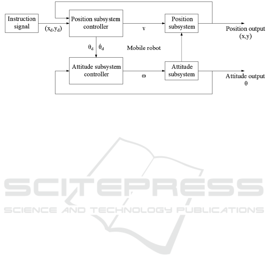
Figure 2: Structure of a closed-loop system with dual loops.
It needs to be explained as follows:
(1) Due to the need to obtain
𝜃
when designing
the inner loop controller, this requires θ
d
to be a
continuous value, thus requiring the control laws u
1
and u
2
to be continuous. Therefore switching
functions should not be included in u
1
and u
2
.
(2) In the control law (20), the intermediate
command signal θ
d
generated by the outer loop needs
to be derived. However, the derivation is too
complicated. For convenience, the following linear
second-order differentiator can be used to obtain
𝜃
[11]:
𝑥
= 𝑥
𝑥
= −2𝑅
𝑥
−𝑛
(
𝑡
)
−𝑅𝑥
𝑦= 𝑥
(23)
Among them, the input signal to be
differentiated is n(t), x
1
is to track the signal, x
2
is the
estimation of the first-order derivative of the signal,
and the initial value of the differentiator is x
1
(0)=0,
x
2
(0)=0. Since the differentiator has an integral chain
structure, when derivation of a signal containing noise
in engineering, the noise is only contained in the last
layer of the differentiator, and the noise in the first
derivative of the signal can be more fully suppressed
by integrating.
(3) In the inner and outer loop control, the
dynamic performance of θ tracking θ
d
in the actual
model will affect the stability of the outer loop, which
will affect the stability of the entire closed-loop
control system. For this problem, the literature
(Bertrand, 2011; Jankovic, 1996; Amit, 2010; Amit,
2010 ) gives a strict solution is proposed, in which the
literature (Bertrand, 2011) deduces the relationship
between the control gains between the inner and outer
loops, thus guaranteeing strict closed-loop system
stability.
In order to achieve stable inner loop sliding
mode control, this section introduces the method
generally used in engineering, that is, the method that
the inner loop convergence speed is greater than the
outer loop convergence speed, and the stability of the
closed-loop system is ensured by θ fast tracking θ
d
. In
this algorithm, by adjusting the control gain
coefficients of the inner and outer loops, the
convergence speed of the inner loop is guaranteed to
be much faster than that of the outer loop, but this
method is only an empirical method, which cannot
theoretically guarantee the stability of the closed-loop
system.
5 SIMULATION EXAMPLE AND
CONCLUSION
5.1 Aperiodic Trajectory
The controlled object is equation (20), and the pose
instruction
𝑥
𝑦
is x
d
=t, y
d
=sin(0.5x)+0.5x+1.
Take k
1
=k
2
=0.30, k
3
=3.0, η
3
=0.50, the initial value of
the pose is
000
, adopt the control law formula
(18) and formula (20), for the switching of the attitude
control law formula (20) term, the saturation function
is used instead of the switching function, the thickness
of the boundary layer is set to 0.10, and the
differentiator parameter is set to R=100. The
simulation results are shown in Figures 3(a)~(d).
It can be seen from the simulation that the
maximum value of θ
d
is 0.9526rad, which belongs to
the interval (-π/2, π/2) and meets the requirements of
formula (17). It can be seen that there is a good
tracking effect for the values in this range.
ICDPCS 2023 - The International Conference on Data Processing, Control and Simulation
92

(a) Tracking of trajectory (b) Tracking of position and angle
(c) Input and output of the differentiator (d) Control input signals v and ω.
Figure 3: The simulation results of aperiodic trajectory.
(a) Tracking of trajectory (b) Tracking of position and angle
(c) Input and output of the differentiator (d) Control input signals v and ω.
Figure 4: The simulation results of periodic trajectory.
0 5 10 15 20 25 30
x
0
2
4
6
8
10
12
14
16
18
ideal trajectory
position tracking
0 5 10 15 20 25 30
time(s)
-8
-6
-4
-2
0
2
4
d
d
d
0 5 10 15 20 25 30
time(s)
1
1.2
1.4
1.6
1.8
0 5 10 15 20 25 30
time(s)
-10
-5
0
0 5 10 15 20 25 30
time(s)
0
50
ideal x
x tracking
0 5 10 15 20 25 30
time(s)
0
5
10
ideal y
y tracking
0 5 10 15 20 25 30
time(s)
-1
0
1
d
d
tracking
Design of Double-Loop Trajectory Tracking Control System for Mobile Robot
93

5.2 Periodic Trajectory
The periodic trajectory mentioned here is generally
more commonly used in trajectory planning, and a
more complex periodic trajectory function is defined
here to verify the practicability of the algorithm. The
pose instruction
𝑥
𝑦
is x
d
=2t-sin(t), y
d
=6-
5cos(t). Take k
1
=k
2
=0.30, k
3
=3.0, η
3
=0.50, the initial
value of the pose is
000
, the thickness of the
boundary layer is set to 0.10, and the differentiator
parameter is set to R=100. The simulation results are
shown in Figures 4(a)~(d). Finally obtained θ
d
is
1.2476rad and still meet the requirements.
If it exceeds this range, given a continuous
trajectory function, it can be seen from equation (17)
that there must be a point in the tracking trajectory
that makes 𝜃
= ∞, so that the robot The tracking
curve of v and ω appears faulty, and the movement of
the robot will be stuck and incoherent. Therefore,
special attention should be paid to the design.
ACKNOWLEDGEMENT
The authors gratefully acknowledge the support of the
National Natural Science Foundation of China (no.
51675315).
REFERENCES
Qu D 2015 Proceedings of the Chinese Academy of
Sciences (3) 342-346.
Tan M, Wang S 2013 Journal of Automatio 39(7) 963-972.
Hu S, Song C 2016 Science and Technology Economics
Guide (10).
Liu T, Gong A, Song C and Wang Y 2020 Energies 13 1029.
Feng J, Zhang W 2017 Information and Control 46(4) 385-
393.
Zhao T, Wang Y 2020 Micromotor 53(1) 111-112, 116.
Chang J, Zhang L, Xue D 2015 Journal of Jiamusi
University(Natural Science Edition) 33(6) 844-847,
928.
Zheng W, Li Y 2017 Computer Engineering and Design
38(2) 539-543.
Zhang L 2019 High-tech Communications 29(6) 607-613.
Tsuchida Y, Oya M, Takagi N, et al 2009 Artificial Life &
Robotics 14(3) 357-361.
Liu T, Zhao K, Sun C, Jia J and Liu G 2020 Energies 13
5029.
Bertrand S, Guenard N, Hamel H, Lahanier H, Eck L 2011
Control Engineering Practice 19 1099-1108.
Jankovic M, Sepulchre R, Kokotovic P, Constructive L
1996 IEEE Transactions on Automatic Control 41(12)
1723-1735.
Amit A 2010 IEEE Transactions on Automatic Control
55(3) 737-743.
Amit A, Llan Z 2010 IEEE Transactions on Automatic
Control 1563-1568.
ICDPCS 2023 - The International Conference on Data Processing, Control and Simulation
94
