Schedulling Production Based on an Optimized Production Sequencer

and Manufacturing Maps

Nuria Rosillo Guerrero

1 a

, Nicol

as Mont

es S

anchez

1 b

, Antonio Falc

o Montesinos

1 c

Eduardo Garcia Magraner

2 d

and Judith Vizcaino Hilario

2 e

Department of Mathematics, Physics and Technological Sciences, University CEU Cardenal Herrera,

C/ San Bartolome 55, 46115 Valencia, Alfara del Patriarca, Spain

Ford Spain, Poligono Industrial Ford S/N, 46440 Valencia, Almussafes, Spain

Keywords:

Industry 4.0, Manufacturing Maps, Petri Nets, Miniterms, Optimal Pathﬁnding Algorithm, Optimal

Manufacturing Sequence.

Abstract:

In this article, we present an innovative application of manufacturing maps, speciﬁcally combining Petri Nets

and Miniterms. Our proposed algorithm enables the determination of an optimal manufacturing sequence

based on real-time information from the manufacturing line. The primary objective of this algorithm is to

minimize the disparity in cycle times between different models, aiming to minimize the duration of worksta-

tions being stopped or blocked. This optimization leads to a reduction in total production time, accompanied

by various beneﬁts such as energy savings and increased production. To validate our approach, we imple-

mented the algorithm using manufacturing maps and applied it to the 8XY line—a multimodel welding line

located at the Ford factory in Almussafes, Valencia. We conducted simulations using actual production data

from the Ford factory, considering three different types of order: random, optimal, and unfavorable. The goal

was to compare the production time for each sequence. The results obtained from the simulations demon-

strated a signiﬁcant time improvement when employing the optimal sequence, as outlined in the article. A

comprehensive analysis of the three sequences studied is provided. As a future direction of this research,

we intend to explore additional applications that can leverage manufacturing maps for production line opti-

mization. For instance, we plan to investigate the determination of optimal sequences for anomalies, where

improvements in the line to reduce cycle time could yield greater proﬁtability. Moreover, we aim to explore

how production lines can be dynamically rebalanced in real-time to achieve energy savings and other advan-

tages. These potential extensions highlight the versatility and practical implications of manufacturing maps in

enhancing production line efﬁciency.

1 INTRODUCTION

Within the framework of Industry 4.0, the landscape

of traditional manufacturing processes is undergo-

ing a profound transformation driven by digitaliza-

tion and advanced technologies. Industry 4.0 rep-

resents a paradigm shift characterized by the exten-

sive adoption of state-of-the-art tools such as artiﬁ-

cial intelligence (AI), the Industrial Internet of Things

(IIoT), and big data analytics, fundamentally altering

the landscape of goods and services production and

https://orcid.org/0000-0002-8935-1581

https://orcid.org/0000-0002-0661-3479

https://orcid.org/0000-0001-6225-0935

https://orcid.org/0000-0002-4210-9835

https://orcid.org/0000-0002-8161-6207

delivery (Schwab, 2016).

Central to Industry 4.0 lies the optimization of

production scheduling, a fundamental facet of man-

ufacturing operations. The convergence of Big Data

and IIoT has ushered in a revolutionary era in pro-

duction scheduling, marked by dynamic scheduling

strategies that permit real-time adjustments in produc-

tion schedules to align with ﬂuctuating conditions and

demands. (Jiang et al., 2022)

The marriage of Big Data analytics with schedul-

ing systems introduces the concept of predic-

tive maintenance, effectively minimizing disruptions

stemming from unforeseen equipment failures (Liu

et al., 2023).

This strategic focus on Scheduling production

within the Industry 4.0 paradigm holds the promise

Rosillo Guerrero, N., Montés Sánchez, N., Falcó Montesinos, A., Garcia Magraner, E. and Vizcaino Hilario, J.

Schedulling Production Based on an Optimized Production Sequencer and Manufacturing Maps.

DOI: 10.5220/0012155300003543

In Proceedings of the 20th International Conference on Informatics in Control, Automation and Robotics (ICINCO 2023) - Volume 2, pages 273-280

ISBN: 978-989-758-670-5; ISSN: 2184-2809

273

of substantial advantages. These encompass cost re-

duction, heightened operational efﬁciency, enhanced

productivity, reduced errors, and bolstered security

(Ghobakhloo, 2020). Furthermore, the amalgamation

of these technologies contributes to sustainability ef-

forts and bolsters environmental preservation.

Despite the undeniable beneﬁts, the implementa-

tion of Industry 4.0 and advanced scheduling solu-

tions is not without its challenges. Concerns span cy-

bersecurity vulnerabilities (Rajalingham, 2020), skills

and training deﬁcits (Bauernhansl et al., 2014), inter-

operability issues (Wang et al., 2016), and substantial

initial investments (Bauernhansl et al., 2014).

In this transformative landscape, sensorization, as

a critical component of IIoT (Peinado-Asensi et al.,

2023a), plays a pivotal role in redeﬁning how pro-

duction scheduling is executed using the philosophy

and the results of our previous works (Garcia, 2022;

Llopis, 2022). By enabling real-time data collec-

tion from various operational facets, sensorization

empowers decision-makers with essential insights to

optimize Production Scheduling processes efﬁciently.

However, sensorization in IIoT is not without its chal-

lenges, including managing and analyzing vast vol-

umes of data, industrial cybersecurity, and interoper-

ability between systems and devices (Peinado-Asensi

et al., 2023b).

1.1 Previous Works

In our previous works, (Peinado-Asensi et al., 2023a;

Peinado-Asensi et al., 2023b), a new concept for gen-

erating industrializable IIoT applications, called In-

dustrializable Industrial Internet of Things (I3oT )

was presented. As we brieﬂy explain in the introduc-

tion, there is an important limitation that is signiﬁ-

cantly slowing down its massive proliferation in the

IIoT application industry. The installation of sensors,

their wiring and data extraction through the IT net-

work to the OT network, and the increasing number

of machines or components to be sensorized prevent

the proposed solutions from being applied in the in-

dustry in a massive way, due to the high cost involved

in their implementation. The idea of the (I3oT ) is to

use the installation available in factories to develop

IIoT applications from them. The machines installed

in the industry operate automatically and have sen-

sors that provide the information received by the PLC

to control the lines.

1.1.1 Miniterm-Based Big Data for Predictive

Maintenance

Previous works carried out by the research group

following the (I3oT ) philosophy was in (Garcia,

2022)where we have presented an innovative solu-

tion for the early detection of faults in industrial ma-

chinery by using a virtual sensor called Mini-term de-

ﬁned in (Garc

ıa, 2016), see ﬁgure 1. The mathemat-

ical model proposed in (Garc

ıa, 2016) was reformu-

lated in (Garc

ıa and Mont

es, 2017), by using tensor

algebra, which reduces the computational cost of the

model, especially when the number of mini-terms and

micro-terms is high. The Miniterm is based on the

measurement of the technical cycle time as a param-

eter to predict failure. When the component is ap-

proaching the end of its useful life, the cycle time in-

creases alerting that it must be replaced. The great ad-

vantage of the miniterm is that it does not require the

installation of any additional sensor, but uses the sen-

sorization of the machine’s own automatic system and

only requires the programming of a timer in the PLC.

In (Garcia, 2022) a case study was presented in which

the Miniterm was implemented in a production line of

a vehicle manufacturing company, in particular, in the

Ford factory based in Almussafes (Valencia). In this

factory there are more than 24,000 mini-terms moni-

toring cylinders, clamps, elevators, screwdrivers, etc.

The results showed that the virtual sensor could de-

tect anomalies, which allowed the maintenance team

to take preventive measures in order to avoid the stop-

page of the production line. This fact has made that

different indicators of the plant, among which is the

TAV (Technical Availability), increased signiﬁcantly,

see (Garcia, 2022).

Figure 1: From the micro-term to the long-term.

1.1.2 Manufacturing Maps for Smart Factory

Management

In the study by (Llopis, 2022) a new tool called Man-

ufacturing Maps is described which is a smart fac-

tory management tool that relies on the combination

of Petri nets and big data mini-terms.

A manufacturing map is a hierarchical construc-

tion of Petri nets in which the lowest level net is a

temporary Petri net based on mini-terms, and in which

the highest level is a global view of the entire plant.

The manufacturing map is fed by Big Data based on

miniterms, which allows it to have in real time the

ICINCO 2023 - 20th International Conference on Informatics in Control, Automation and Robotics

274

current status of the components that make up the pro-

duction chain, see ﬁgure 2

Figure 2: From the micro-term to the long-term in a Manu-

facturing Map

Once the petri net model is built, the user of the

Manufacturing Map can select which view of the

plant he/she wants, being able to select the lowest

level view, machine view, or a global view of the

plant, commodity view. The navigation through the

different levels is done as in google maps, see (Llopis,

2022).

2 OUTLINE OF OBJECTIVES

The previous modelling and simulation work of the

Manufacturing Maps, combined with the real-time

measurements of the miniterms can generate count-

less new applications. The present article seeks to ex-

plore one such application, namely, to seek the opti-

mal manufacturing sequence in real time in order to

minimize manufacturing time.

This objective is one of the topics explored in the

literature, as for example in (Jiang et al., 2018), in

which a production programming system based on the

Internet of Things (IoT) was proposed in order to op-

timize the production sequence in real time. The sys-

tem used sensors and IoT devices to collect real-time

data on production and quality, and then used opti-

mization algorithms to generate the optimal manufac-

turing sequence. In this article, Manufacturing Maps

(Petri nets + Miniterms) will be used to generate the

optimal manufacturing sequence based on the current

state of the line measured with the miniterms. With-

out loss of generality, the present article focuses on

the optimization of manufacturing sequences for the

automotive sector where the use of ﬂexible manufac-

turing lines is quite widespread.

3 METHODOLOGY

3.1 Ordering a Production Stack

When ordering a Production Stack for the automotive

sector, we start from the fact that our stack will in-

clude the vehicles to be produced. Not all vehicles are

the same, there are different models of the same ve-

hicle with different characteristics. The same model

can have 3 or 5 doors, may or may not have a sunroof,

etc., which generates signiﬁcant variability between

models. Let’s deﬁne {1...m} as the different models

or variants.

The manufacturing line will be composed of

workstations and where in each of them a speciﬁc

work will be carried out to manufacture the vehicle.

We assume in this case that we will have {1...n} work-

stations on the manufacturing line on which the order-

ing of the production stack will be carried out.

Be a

i, j

the TcT (Cycle Time) of the model i in the

station j. We can consider matrix W as the matrix that

provides us with information about the Cycle Times

(TcT) of each model (rows) at each station (columns).

i, j







1,1

1,2

. . . a

1,n

2,1

2,2

. . . a

2,n

m,1

m,2

. . . a

m,n







(1)

From this matrix, we can obtain two types of ma-

trices, the matrix of minimum weights and/or the ma-

trix of maximum weights, which will allow us to de-

termine the most favourable and unfavourable order-

ing possible.

3.1.1 Minimum Weights Matrix

We start from the M matrix calculated above and we

want to ﬁnd the lowest diference TcT between differ-

ent models or rows of the M matrix.

We will get a matrix N of mxm where each ele-

ment n

i, j

as the minimum absolute value of the differ-

ence between the elements of the row i and the row

N(i, j) = min |M(i, k) − M( j, k)| (2)

for all k=1,2,...,n

This new N matrix will enable us to identify the

shortest Cycle Time (TcT) among various models or

rows in the N matrix. Each element of the textitN ma-

trix represents the minimum variation between rows i

and j in the M matrix.

Schedulling Production Based on an Optimized Production Sequencer and Manufacturing Maps

275

i, j







1000 n

1,2

. . . n

1,m

2,1

1000 . . . n

2,m

m,1

m,2

. . . 1000







(3)

3.1.2 Algorithm for Determining Optimal

Ordering Sequence

• Initialization: The initial element of the optimal

ordering sequence is identiﬁed as the row contain-

ing the ﬁrst model to be manufactured.

• Second Element: The second element of the opti-

mal ordering sequence corresponds to the column

associated with the ﬁrst element in the sequence.

• Iterative Process: To determine the remaining el-

ements of the optimal ordering sequence, we fol-

low an iterative process:

. Selection: From the set of remaining mod-

els (m-2), we select the row that corresponds to

the column of the previous element in the optimal

sequence.

Minimum Search: Subsequently, we identify

the minimum value within that selected row.

Next Element: The column corresponding to

this minimum value is designated as the next ele-

ment in the optimal ordering sequence.

• Completion: We repeat this iterative process un-

til all elements of the optimal ordering sequence

have been determined.

This algorithmic approach facilitates the systematic

determination of the optimal ordering sequence for

the manufacturing process according to their mini-

mum total cycle time (TcT).

3.1.3 Maximum Weights Matrix

During the comparison of production times based on

different orderings, we conducted an analysis that

aimed to maximize the Cycle time (TcT), focusing

on the worst-case scenario. This particular ordering

strategy is built upon a weighted matrix, in which we

calculate the largest TcT when transitioning from one

model to another.

Our starting point is the previously computed ma-

trix M, and our objective is to identify the maxi-

mum TcT difference between various models or rows

within matrix M.

D(i, j) = max |M(i, k) − M( j, k)| (4)

for all k=1,2,...,n

To achieve this, we construct a matrix D with di-

mensions mxm, where each element d

i, j

represents

the maximum absolute difference in TcT between row

i and column j in matrix M.

i, j







−1 d

1,2

. . . d

1,m

2,1

−1 . . . d

2,m

m,1

m,2

. . . −1







(5)

This approach allows us to effectively maximize

the TcT difference among the different models to be

produced, all of which are represented by the rows

within matrix D.

3.1.4 Algorithm for Determining the Most

Unfavorable Sequence of Manufacturing

Models

To identify the most unfavorable sequence for the pro-

duction of various models, we begin with the ma-

trix D, which encapsulates the maximum Cycle time

(TcT) incurred when transitioning between different

models during manufacturing.

The procedure for ﬁnding this sequence closely

parallels the method used to identify the most favor-

able sequence:

• Initialization: We commence by selecting the

ﬁrst element of the most unfavorable ordering se-

quence, which corresponds to the row containing

the ﬁrst model to be manufactured.

• Second Element: The second element of this se-

quence corresponds to the column associated with

the ﬁrst element selected.

• Iterative Process: To determine the remaining ele-

ments of the most unfavorable ordering sequence,

we employ an iterative process:

Selection: From the set of remaining (m-2)

models, we choose the row corresponding to the

column of the preceding element in the sequence.

Maximum Search: Subsequently, we iden-

tify the maximum value within that selected row.

Next Element: The column corresponding to

this maximum value is designated as the next ele-

ment in the sequence.

• Completion: We repeat this iterative process until

all elements of the ordering sequence have been

determined.

As a result, this algorithm produces a vector rep-

resenting the most unfavorable sequence for ordering

different models based on their accumulated maxi-

mum total cycle time (TcT).

ICINCO 2023 - 20th International Conference on Informatics in Control, Automation and Robotics

276

4 EXAMPLE OF APPLICATION

ON A REAL LINE

4.1 Deﬁnition of the Welding Line and

the Manufacturing Maps Model

Previous works by the (Llopis, 2022) research group

have used the welding line as an example, which is a

line of multiple models where 68 different models and

variants are manufactured. The line consists of eight

workstations where three of them have six welding

units, four stations have four welding units and one

station has a welding unit as shown in Figure 3.

The Petri net is built from real-time information

of three mini-terms at each station, which measure

the sub-cycle time for robot arm movement, welding

clamp movement and welding task. The welding line

is modelled from the plane of view of the manufac-

turing map line and divided into three layers: the A

layer shows the eight stations connected in series, the

B layer covers each station with six, four or one weld-

ing unit, and the C layer models the process of a di-

vided welding unit in its mini-terms as seen in Figure

There are two ways to interpret process modelling

by using the Petri net: considering transitions as ac-

tions and places as states, or considering transitions as

a set of actions and places as states. In this case, the

transition is understood as an action and an example

of substitution transition is used to introduce subnets

into the hierarchical network.

Once the modelling of the main Petri net corre-

sponding to the A layer has been carried out, each of

the transitions is deepened in a subnet that includes

all the actions carried out within the corresponding

station. Each subnet contains subnets, which gives

the hierarchical network a deeper structure. In each

subnet corresponding to a station, there is a transition

including a subnet for each robot.

The C layer is fed directly by the Miniterms Big

Data, in which sub-cycle times are available for the

robot arm movement, the welding clamp movement

and the welding task in real time. The A layer model

is obtained by the ﬂattening technique, see (Llopis,

2022).

4.2 Data

When performing the simulation of the welding line,

the ﬁrst thing to be done is the generation of the

production stack, in our case the stack has a size of

10,000 vehicles. The generation of the production

stack is based on the actual production of the Ford fac-

tory in Almussafes in March 2015, from these produc-

tion data the probability of manufacturing each of the

models is calculated and the 10,000 cars to be man-

ufactured are generated with their different models

based on the previously calculated probability. The

actual production stack is not random since it is based

on the processing of orders placed at the factory, but

depending on the orders there is no speciﬁc sorting

sequence so it could be considered random.

4.3 Production Stack Ordering

In order to carry out a comparative study of the pro-

duction time, which is the time used to manufacture

the same production stack, three types of ordering of

the production stack have been carried out:

• Random sequence, the manufacturing sorting se-

quence is completely random and is based on the

fact that it is manufactured according to the order

placed so it is also considered random.

• Optimal ordering based on the minimum path pre-

viously explained.

• Unfavourable ordering, this type of ordering is

based on the maximum path explained in the pre-

vious point.

4.3.1 The Most Favourable Sequence

This type of ordering is completely straightforward,

we take the optimal ordering sequence and the vector

to be ordered (Production Stack) and return the or-

dered vector according to the optimal sequence. One

of the characteristics of this sequence is that those

same models are manufactured together, that is, the

set of vehicles belonging to the same model are man-

ufactured in a block (one after another).

4.3.2 The Most Unfavourable Sequence

The function implemented to sort the production

stack, as in the optimal sequence, uses an iterative ap-

proach that follows the previously obtained optimal

sorting path.

Each element of the production stack is checked

one by one, in each iteration of the loop, the current

element of the production stack is compared with the

elements of the optimal ordering sequence according

to the established maximum. If they are equal, the

next element of the optimal sequence is saved and that

next element is searched in the Production Stack and

if it is found, it is added to the ordered Stack and re-

moved from the Production Stack. If not found, the

current Production Stack item is added to the sorted

Stack.

Schedulling Production Based on an Optimized Production Sequencer and Manufacturing Maps

277

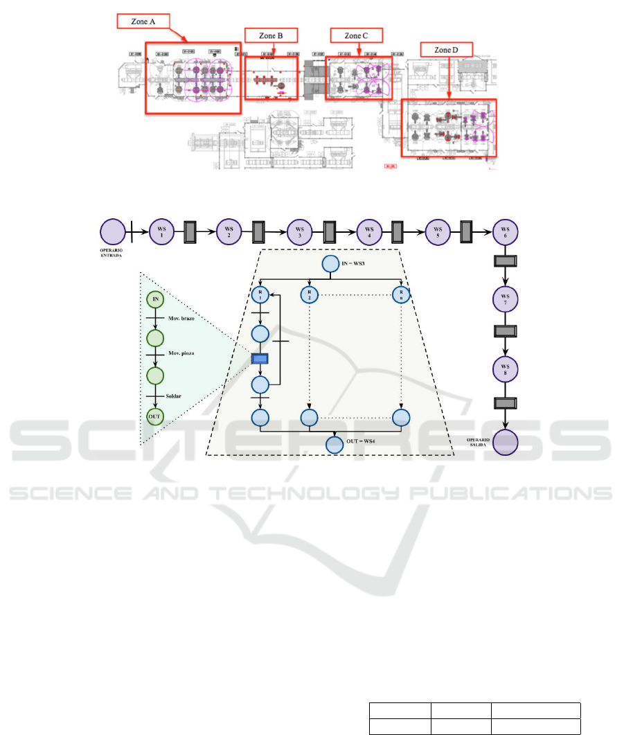
Figure 3: Layout welding line.

Figure 4: Hierarchical Petri net of the 8XY line.

At the end, the function returns the vector with

the sorted stack, which contains the elements of the

Production Stack ordered according to the optimal se-

quence with a set maximum. The reason why this

type of ordering is carried out is because we do not

want vehicles of the same model one after the other,

that is, behind a speciﬁc vehicle will always follow

the one that has a worse time, therefore, the most un-

favourable one.

4.4 Results

Once we have implemented the simulation of the

welding line with the Petri nets and the production

data based on the real production of the Ford factory

in Almussafes that we use to simulate the manufacture

of 10,000 cars, we proceed to simulate said manufac-

ture. The same Production Stack will be simulated

with the 3 ordering sequences described above:

• Random

• Optimal

• Unfavourable

As seen in ﬁgure 5, we have generated 25 differ-

ent data sets (production stacks), using the manufac-

turing probability from the month of March 2015 and

we have simulated them using the three pre-set sorting

sequences in order to obtain a more detailed analysis

of production times and obtain more precise and reli-

able results. As a summary of the previous ﬁgure, we

can calculate the average production times in hours

of the 25 stacks generated with each of the ordering

sequences studied as shown in table1:

Table 1: Average production time according to the ordering

sequence in hours.

Random Optimal Unfavourable

306.40 291.35 314.49

As seen in table 1, the production time is being im-

proved if the production stack is ordered. Next, we go

on to comment in more detail on the results obtained.

ICINCO 2023 - 20th International Conference on Informatics in Control, Automation and Robotics

278

Figure 5: Results.

5 DISCUSSION

In view of the results obtained in the previous sec-

tion, we can observe an improvement in production

times when ordering the stack of cars to be manu-

factured following the optimal sequence based on the

minimum accumulated TcT.

In this way we can study how much we are im-

proving with respect to the random sequence of the

production stack and we can also compare the data

with the most unfavourable sequence.

From these data we have studied the percentage

of improvement in production times for 10 of the 25

production stacks generated as shown in table 2:

Table 2: Percentages of improvement ordering the produc-

tion according to optimal sequence.

Production Stack Improvement percentages

Stack 1 5.0%

Stack 2 5.1%

Stack 3 4.9%

Stack 4 5.5%

Stack 5 5.3%

Stack 6 5.0%

Stack 7 5.3%

Stack 8 5.2%

Stack 9 4.3%

Stack 10 5.3%

If we calculate the average percentage of improve-

ment by ordering the production stack with the op-

timal sequence, there is an average improvement of

about 5.1% of the production time, which means that

in the case of manufacturing 10,000 cars, 5.1% ex-

tra cars could be produced in the same time, which is

equivalent to producing 510 extra cars.

In the case of studying the worst possible case,

which means that we are ordering following the most

unfavourable sequence without the possibility of car

model repetition, the results would be as follows com-

paring the worsening with respect to the ordering with

the optimal sequence as shown in table 3 and with the

production stack using a random order as shown in

table 4.

Table 3: Worsering percentages ordering the production ac-

cording to optimal sequence.

Production Stack Worsening percentages

Stack 1 8.1%

Stack 2 8.7%

Stack 3 8.0%

Stack 4 5.8%

Stack 5 7.7%

Stack 6 8.0%

Stack 7 7.7%

Stack 8 7.8%

Stack 9 8.3%

Stack 10 7.8%

If we calculate from table 3 the average percent-

age of production time that is getting worse if we

compare with the optimal sequence, we observe that

the average percentage is 7.8%, which means that in

the same time we are manufacturing about 780 fewer

vehicles if we compare with the optimal sequence.

Schedulling Production Based on an Optimized Production Sequencer and Manufacturing Maps

279

Table 4: Worsening percentages ordering the production ac-

cording to random sequence.

Production Stack Worsering percentages

Stack 1 2.6%

Stack 2 3.1%

Stack 3 2.7%

Stack 4 2.7%

Stack 5 2.3%

Stack 6 2.7%

Stack 7 2.3%

Stack 8 2.3%

Stack 9 2.9%

Stack 10 2.4%

In this case the production time worsens on av-

erage by 2.6% when compared to the random pro-

duction stack, actually the percentage is not very high

compared to the randomization. The results show us

that the improvement in production time when order-

ing the production stack from an optimal sequence

based on the minimum accumulated TcT between the

different models is signiﬁcant.

6 CONCLUSIONS

In this article we have proposed an application to

manufacturing maps (Petri Nets+Miniterms) by gen-

erating an algorithm that allows to determine the opti-

mal manufacturing sequence with the real-time status

of the manufacturing line. As demonstrated in this

article, there is a considerable gain in time. In our

future works we will try to study new applications

that manufacturing maps can offer for the optimiza-

tion of production lines such as, for example, ﬁnding

out the optimal sequence for an anomaly, where could

be more proﬁtable the applications of improvements

in the line to reduce cycle time or how to rebalance in

real time the lines to save energy, etc.

ACKNOWLEDGEMENTS

Authors wish to thank Almussafes factory for the help

in the development of the present study.

REFERENCES

Bauernhansl, T., ten Hompel, M., and Vogel-Heuser, B.

(2014). Industrie 4.0 in Produktion, Automatisierung

und Logistik. Springer.

Garc

ıa, E. (2016). An

alisis de los sub-tiempos de ci-

clo t

ecnico para la mejora del rendimiento de las

ıneas de fabricaci

on. PhD thesis, Universidad CEU-

Cardenal Herrera, Alfara del Patriarca, Spain.

Garc

ıa, E. and Mont

es, N. (2017). A tensor model for au-

tomated production lines based on probabilistic sub-

cycle times. In Modeling Human Behaviour: Individ-

uals and Organization, pages 221–234. Nova Science

Publishers, Hauppauge, NY, USA.

Garcia, E. (2022). Miniterm, a novel virtual sensor for pre-

dictive maintenance for the industry 4.0 era. Sensors,

22(1):100.

Ghobakhloo, M. (2020). Industry 4.0, digitization, and op-

portunities for sustainability. Journal of Cleaner Pro-

duction, 252:119869.

Jiang, S., Li, X., and Chen, Y. (2018). A real-time produc-

tion scheduling system based on the internet of things

for industry 4.0. Journal of Intelligent Manufacturing,

29(4):935–948.

Jiang, Z., Yuan, S., Ma, J., and Wang, Q. (2022). The

evolution of production scheduling from industry 3.0

through industry 4.0. International Journal of Pro-

duction Research, 60(11):3534–3554.

Liu, L., Song, W., and Liu, Y. (2023). Leveraging digital

capabilities toward a circular economy: Reinforcing

sustainable supply chain management with industry

4.0 technologies. Computers & Industrial Engineer-

ing, 178:109113.

Llopis, J. (2022). Manufacturing maps, a novel tool for

smart factory management based on petri nets and big

data mini-terms. Mathematics, 10(14):2398.

Peinado-Asensi, I., Mont

es, N., and Garc

ıa, E. (2023a). Vir-

tual sensor of gravity centres for real-time condition

monitoring of an industrial stamping press in the au-

tomotive industry. Sensors, 23(14).

Peinado-Asensi, I., Mont

es, N., Iba

nez, D., and Garc

ıa, E.

(2023b). Industrializable industrial internet of things

(i3ot ). a press shop case example. International Jour-

nal of Production Research.

Rajalingham, K. (2020). Cybersecurity in industry 4.0: An

overview. Journal of Information Security and Cyber-

crimes, 4(1):1–8.

Schwab, K. (2016). The Fourth Industrial Revolution.

Crown Business, London, 2nd edition.

Wang, X., Wan, J., Zhang, D., Li, D., and Zhang, C.

(2016). Towards smart factory for industry 4.0: a

self-organized multi-agent system with big data based

feedback and coordination. Computer Networks,

101:158–168.

ICINCO 2023 - 20th International Conference on Informatics in Control, Automation and Robotics

280