Real-World Optimization Benchmark from Vehicle Dynamics:

Speciﬁcation of Problems in 2D and Methodology for Transferring

(Meta-)Optimized Algorithm Parameters

Andr

e Thomaser

1,2 a

, Marc-Eric Vogt

1 b

, Thomas B

ack

2 c

and Anna V. Kononova

2 d

BMW Group, Knorrstraße 147, Munich, Germany

LIACS, Leiden University, Niels Bohrweg 1, Leiden, The Netherlands

Keywords:

Parameter Tuning, CMA-ES, Vehicle Dynamics Design, Benchmarking, Exploratory Landscape Analysis,

Artiﬁcial Benchmarking Functions.

Abstract:

The algorithm selection problem is of paramount importance in achieving high-quality results while minimiz-

ing computational effort, especially when dealing with expensive black-box optimization problems. In this

paper, we address this challenge by using randomly generated artiﬁcial functions that mimic the landscape

characteristics of the original problem while being inexpensive to evaluate. The similarity between the artiﬁ-

cial function and the original problem is quantiﬁed using Exploratory Landscape Analysis. We demonstrate

a signiﬁcant performance improvement on ﬁve real-world vehicle dynamics problems by transferring the pa-

rameters of the Covariance Matrix Adaptation Evolution Strategy tuned to these artiﬁcial functions.

We provide a complete set of simulated values of braking distance for fully enumerated 2D design spaces

of all ﬁve real-world optimization problems. So, replication of our results and benchmarking directly on the

real-world problems is possible. Beyond the scope of this paper, this data can be used as a benchmarking set

for multi-objective optimization with up to ﬁve objectives.

1 INTRODUCTION

Optimization algorithms play a vital role in solv-

ing complex real-world problems in a variety of do-

mains, including engineering, ﬁnance, logistics, and

machine learning. Evaluating and comparing these

algorithms is critical to selecting the best approach

for a given (class of) problem(s). This means running

multiple full optimizations. Since real-world prob-

lems are often comparatively expensive, this can be

archived by running the different algorithms on stan-

dardized, well-deﬁned benchmark problems. While

these benchmark problems, such as the black-box op-

timization benchmark suit (BBOB) (Hansen et al.,

2009), are inexpensive to evaluate, they often cannot

fully capture the intricacies and complexities present

in real-world scenarios. Randomly generated artiﬁ-

cial functions can be used to create more similar prob-

lems (Long et al., 2022).

https://orcid.org/0000-0002-6210-8784

https://orcid.org/0000-0003-3476-9240

https://orcid.org/0000-0001-6768-1478

https://orcid.org/0000-0002-4138-7024

The Covariance Matrix Adaptation Evolution

Strategy (CMA-ES) (Hansen, 2016; Hansen and

Ostermeier, 1996) is a class of iterative heuris-

tic algorithms and is considered as state-of-the-

art in single objective, continuous black-box opti-

mization, with many successful real-world applica-

tions such as topology optimization (Fujii et al.,

2018) and hyperparameter optimization of neural net-

works (Loshchilov and Hutter, 2016). Many vari-

ants have been developed over the years. The task

of identifying and selecting the variant with the best

performance for a given problem is a key challenge

and is known as the algorithm selection problem

(ASP) (Rice, 1976).

In this paper, we present ﬁve real-world 2D op-

timization problems from vehicle dynamics (Sec-

tion 2). We have computed all possible combina-

tions of the two enumerated design parameters. Thus,

this set of values allows the replication of our results

and benchmarking directly on the real-world prob-

lems. In the next step, we generate many suitable

artiﬁcial functions and select the most similar ones

to each real-world problem in terms of Exploratory

Thomaser, A., Vogt, M., Bäck, T. and Kononova, A.

Real-World Optimization Benchmark from Vehicle Dynamics: Speciﬁcation of Problems in 2D and Methodology for Transferring (Meta-)Optimized Algorithm Parameters.

DOI: 10.5220/0012158000003595

In Proceedings of the 15th International Joint Conference on Computational Intelligence (IJCCI 2023), pages 31-40

ISBN: 978-989-758-674-3; ISSN: 2184-3236

Landscape Analysis features (Section 3). These sim-

ilar functions are then used as a tuning reference to

which the parameters of the optimization algorithm

are tuned before being applied to the original expen-

sive real-world problem. As an optimization algo-

rithm, we use the modular CMA-ES implementation

with several different variants that can be combined

arbitrarily (Section 4). Finally, we compare the per-

formance on the 2D real-world problems of the tuned

CMA-ES parameters on the artiﬁcial functions and

BBOB functions with the directly tuned parameters

on the 2D real-world problems (Section 5).

2 REAL-WORLD PROBLEMS

2.1 Description and Objective

Vehicle dynamics control systems, such as the Anti-

lock Braking System (ABS) (Koch-D

ucker and Pa-

pert, 2014), have revolutionized the automotive in-

dustry by enhancing vehicle safety and performance.

The ABS mitigates the risk of wheel lock-up during

braking, by adjusting the brake pressure to keep brake

slip within an optimal range. This reduces the braking

distance and allows the driver to maintain control and

steer the vehicle even in an emergency braking situa-

tion. The parameters of these control systems must be

carefully calibrated to achieve optimal performance

under different scenarios and vehicle settings.

An industry standard maneuver for evaluating

a vehicle’s braking performance is the emergency

straight-line full-stop braking maneuver with ABS

fully engaged (International Organization for Stan-

dardization, 2007). The maneuver consists of the fol-

lowing three phases (Figure 1):

• 1: Accelerate the vehicle to 103.5 km/h;

• 2: No acceleration or deceleration until 103 km/h;

• 3: Apply brakes until the vehicle stops.

The braking distance can be calculated as the in-

tegral of the vehicle’s longitudinal velocity over time

from v

= 100 km/h at time t

to v

= 0 km/h at time t

(Figure 1). The beginning of the braking process be-

tween 103 km/h and 100 km/h is not taken into ac-

count when calculating the braking distance to avoid

possible disturbances occurring at the beginning of

the braking process. According to ISO 21994:2007,

a measurement sequence for calculating the braking

distance consists of ten valid single measurements.

The braking distance y is deﬁned as:

y =

∑

k=1

(t) dt. (1)

Time t in s

100

Lateral velocity v

in km/h

1 2 3

Figure 1: An emergency straight-line full-stop braking

maneuver for calculating the braking distance from v

100 km/h to v

= 0 km/h (start time t

and end time t

2.2 Simulation Environment

The vehicle dynamics, driver, and environment are

simulated using a two-track model implemented in

Simulink (The MathWorks, Inc., 2015). The vehi-

cle dynamics part includes the mechanical vehicle and

the control systems. The mechanical vehicle is mod-

eled as a ﬁve-body model (car body and four wheels)

with 16 degrees of freedom and consists of the follow-

ing components: equation of motion, tires, drive train,

aerodynamics, suspension, steering, and braking. The

control system components are sensors, logic, and ac-

tuators. By virtually mapping the interaction between

these components, the simulation is able to represent

an integrated control system.

MF-Tyre/MF-Swift (Siemens Digital Industries

Software, 2020), which is based on Pacejka’s so-

called Magic Formula (Pacejka and Bakker, 1992), is

used to accurately simulate the steady-state and tran-

sient behavior of tires under slip conditions. The road

surface is described by a curved regular grid (CRG)

track (VIRES Simulationstechnologie GmbH, 2020),

which provides information about the road width and

elevation along a predeﬁned reference line. CRG

tracks are able to model 3D roads in great detail while

keeping memory usage to a minimum. On a standard

workstation

, it takes about 15 minutes to simulate a

braking maneuver. To reduce the wall clock time, the

simulation is run in parallel on multiple computers.

2.3 Real-World Benchmark-Problems

There are two very important ABS control parame-

ters that have a huge impact on the braking distance,

referred to here as x

and x

. Each parameter has a

deﬁned lower B

and upper B

bounds: x

∈ [−5, 6]

and x

∈ [−5, 4]. Furthermore, for x

and x

only a

HP Workstation Z4 G4 Intel Xeon W-2125

4.00GHz/4.50GHz 8.25MB 2666 4C 32GB DDR4-2666

ECC SDRAM

ECTA 2023 - 15th International Conference on Evolutionary Computation Theory and Applications

Table 1: Explaination of the vehicle settings.

Name Tires Vehicle Load

y1 High performance Partially loaded

y2 Medium performance Partially loaded

y3 Under performance Partially loaded

y4 High performance Fully loaded

y5 High performance Little loaded

set of values D

with a resolution of 0.1 as equal dis-

tance between the values is allowed. This means that

111 distinct values are possible for x

and 91 for x

The 2-dimensional input space D

= ×

i=1

is then

the corresponding cartesian product. Thus there are

10101 possible combinations for the two ABS param-

eters x

and x

By simulating every possible combination (brute

forcing) of the two ABS parameters, we can fully

learn the functional dependence between the two ABS

parameters and the resulting braking distance y(x).

Furthermore, in order to apply algorithms for contin-

uous input spaces, in the following we consider the

problem as quasi-continuous: given an input x ∈ R

within the lower and upper bounds, the correspond-

ing braking distance y(x) is determined by round-

ing x

and x

to the nearest data point within the 2-

dimensional input space D

= ×

i=1

In summary, the objective is to ﬁnd a parameter

setting x that minimizes the simulated braking dis-

tance y(x), as deﬁned by the equation (1):

minimize

x∈X

y(x), X = {x ∈ R

: B

≤ x ≤ B

}. (2)

Generally, an optimal parameter setting x

∗

is only

optimal for one vehicle setting. In this paper, we pro-

vide the data of ﬁve different vehicle settings. Here, a

setting consists of a vehicle load and a tire (Table 1).

Since we are interested in the distance to the

global optimum, all braking distances of a particular

vehicle setting i are speciﬁed as the distance in meters

to the corresponding optimum. Figure 2 shows the

distribution of the 10 101 data points for each real-

world problem yi. The data with additional Python

code for benchmarking has been made available on

our Zenodo repository (Thomaser et al., 2023a).

Note that minimizing the braking distance for

each vehicle setting is one objective. For each ve-

hicle setting respectively objective function, a differ-

ent parameter set (x

, x

) is optimal, and the objec-

tives are in conﬂict with each other. Therefore, the

provided data can be used for benchmarking multi-

objective optimization algorithms with up to ﬁve ob-

jectives. However, in this paper, we focus only on

single-objective optimization and do not investigate

the conﬂict between the different vehicle settings.

0.0 0.5 1.0 1.5 2.0 2.5

Distance to y

i, opt

in m

200

400

600

800

Count

Figure 2: Distribution of the 10 101 data points for each of

the ﬁve vehicle settings yi (Table 1).

3 TUNING REFERENCES

3.1 Benchmark Functions

Benchmarking algorithms is an important practice

that facilitates the evaluation and comparison of al-

gorithm performance. A widely accepted bench-

mark suite for single-objective optimization prob-

lems is the Black-Box Optimization Benchmark

(BBOB) (Hansen et al., 2009).

In addition to the 24 BBOB functions, we

randomly generate 100 000 artiﬁcial functions in

2D. Therefore, we use the Python implementation

of (Long et al., 2022), which is based on (Tian et al.,

2020). The input space is the same as for the ﬁve real-

world problems yi, x

∈ [−5, 6], and x

∈ [−5, 4].

We use the instance-generating mechanism of the

BBOB function suite (Hansen et al., 2009) and con-

sider ﬁve instances of each function. We also ap-

ply the same mechanism four times to each of the

100000 randomly generated artiﬁcial functions to ob-

tain slightly different functions, that are simply ro-

tated and shifted relative to the original function.

Maximizing or minimizing a function has a huge im-

pact on the landscape from the point of view of an op-

timization algorithm, so we also consider the inverse

function (multiplied by -1) of each function. This re-

sults in a set of 1 000 000 different artiﬁcial functions.

3.2 Exploratory Landscape Analysis

To quantify high-level properties, such as global

structure or multi-modality, of the landscape of an

optimization problem we use Exploratory Landscape

Analysis (ELA) (Mersmann et al., 2011; Mersmann

et al., 2010). This allows us to compute the similar-

ity between two optimization problems. The ELA-

features can be computed primarily with a sample of

Real-World Optimization Benchmark from Vehicle Dynamics: Speciﬁcation of Problems in 2D and Methodology for Transferring

(Meta-)Optimized Algorithm Parameters

Figure 3: Scatter plot of the two main PCA components

of the 50 ELA-features for the artiﬁcial functions (AF), the

BBOB functions, and the real-world problems yi.

points of the objective function. The pﬂacco pack-

age (Prager, 2023), which provides a native Python

implementation of the large collection of ELA fea-

tures in the ﬂacco package (Kerschke and Trautmann,

2019). We consider only those ELA features that

can be computed cheaply without additional resam-

pling. This results in 55 individual features, which

are grouped in ﬁve sets: classical ELA (distribution,

level, meta) (Mersmann et al., 2011), information

content (Mu

noz et al., 2015), dispersion (Lunacek

and Whitley, 2006), nearest better clustering (Preuss,

2012; Kerschke et al., 2015) and principal compo-

nent. Five features could not be computed for each

function and were discarded.

As a compromise between accuracy and compu-

tational effort in ELA, a sample size of 50 times

the dimensionality is recommended to classify the

BBOB functions with ELA features (Kerschke et al.,

2016). To increase the accuracy we use a Sobol’ de-

sign (Owen, 1998; Sobol’, 1967) with 1000 samples

(500 × 2). For equal weighting, the feature values are

min-max-scaled to [0, 1]. Overall, the feature calcula-

tion was successful for 99.5% of the randomly gener-

ated artiﬁcial functions. Reasons for unsuccessful cal-

culations are ‘not a number’ values as function values

or a ﬂat ﬁtness function.

A large number of considered features leads to re-

dundancy within the features (

Skvorc et al., 2020).

Therefore, to remove redundant features and reduce

the dimensionality of the feature space, we perform

Principal Component Analysis (PCA) (Jolliffe, 1986).

With the requirement of a cumulative variance greater

than 0.999, the dimensionality of the feature space is

reduced to 31.

Furthermore, Figure 3 shows the position deﬁned

by the two main components from the PCA for each

function considered. The BBOB functions cover only

a partial space. The space in between is ﬁlled with the

Table 2: Most similar BBOB function to each of the real-

world problems yi.

Name Most similar BBOB Function

y1 B

uche-Rastrigin Function f

y2 B

uche-Rastrigin Function f

y3 Weierstrass Function f

y4 Rastrigin Function f

y5 Rastrigin Function f

y1 y2 y3 y4

sim, 1

sim, 2

sim, 3

BBOB

sim

Sphere

0 0.84 6.3 4.3 4.2

0.84 0 6.4 4.2 4.3

6.3 6.4 0 6 6

4.3 4.2 6 0 2.6

4.2 4.3 6 2.6 0

0.95 1.1 1 0.74 1.3

1.1 1.2 1.1 0.91 1.4

1.1 1.2 1.2 1 1.4

2 2 2.9 2.3 2.6

5.1 5.1 7.1 4.2 4.6

Figure 4: Similarity of the landscape (as deﬁned in equa-

tion 3) of the ﬁve real-world problems yi (x-axis) to each

other, the Sphere function (BBOB function f

), the three

most similar artiﬁcial generated functions (AF

sim,i

) and the

most similar BBOB function (BBOB

sim

) for each of the

real-world problems.

randomly generated artiﬁcial functions. The different

vehicle settings of the real-world problem (Table 1)

are relatively widely scattered. This indicates dissim-

ilarities within the landscape of the vehicle settings.

Only y1 and y2 are relatively close to each other.

3.3 Similar Functions

Based on the reduced set of features produced by

PCA, we can quantify the similarity between two

problems p

and p

via the city-block distance d be-

tween their feature vectors F

and F

d(p

, p

) =

∑

− F

. (3)

Using equation 3, we compute the distances be-

tween the ﬁve real-world problems yi and other func-

tions. In the following, we examine the three most

similar randomly generated artiﬁcial functions for

each of the real-world problems, denoted as AF

sim, j

and for comparison also each the most similar BBOB

function and the Sphere function (Table 2). Figure 4

shows these distances, which range from 0.74 to 7.1.

We observe that the distance between y1 and y2

is relatively small with a value of 0.84, for compar-

ison the most similar BBOB function is for both the

uche-Rastrigin function with a distance of 2.0 and

the distances to the other real-world problems y3, y4,

ECTA 2023 - 15th International Conference on Evolutionary Computation Theory and Applications

y5 are always greater than 4 (Figure 4). Thus y1 and

y2 can be considered as similar to each other, while

the other real-world problems are more dissimilar to

y1 and y2 and also to each other.

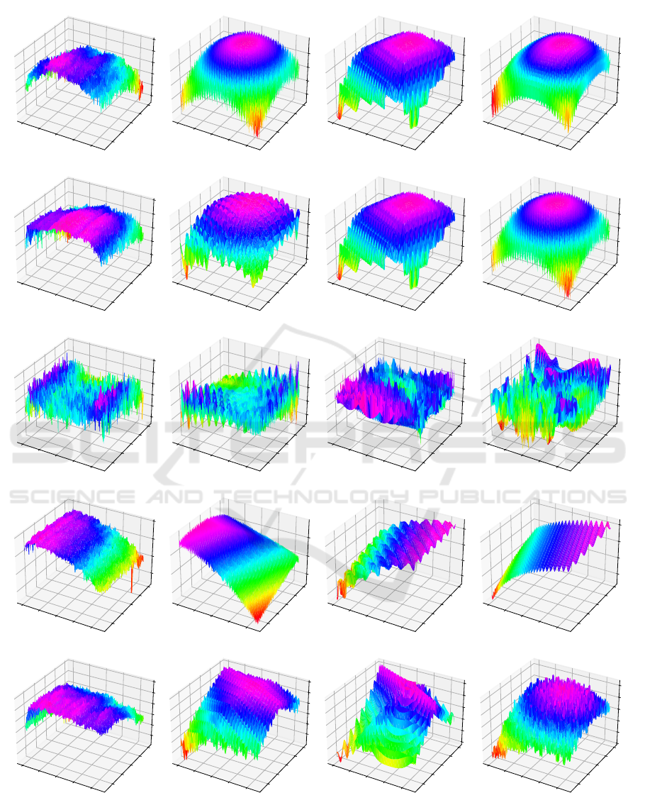
Within the randomly generated artiﬁcial func-

tions, the three most similar to each real-world prob-

lem yi all have a distance between 0.74 and 1.4. Fig-

ure 5 shows the actual landscape of real-world prob-

lems and these most similar artiﬁcial functions. Only

tiny changes within the straight-line braking maneu-

vers can inﬂuence the braking distance, thus all real-

world problems yi are overlaid with noise, which

leads to a highly multi-modal landscape. This noise

or multi-modality is also depicted by the similar arti-

ﬁcially generated functions. Furthermore, we observe

from Figure 5 that, with the exception of y3 (under

performance tires), the real-world problems have a

global structure. This global structure is very similar

for y1 and y2 - as expected from the distance (Fig-

ure 4). The similar artiﬁcially generated functions

also manage to capture such a global structure.

The Sphere function is very dissimilar to the real-

world problems, especially to y3. This is not surpris-

ing, since the Sphere function is uni-modal and does

not capture the noise within the landscape of the real-

world problem. In the following, the Sphere function

will be used as an example of a dissimilar function for

comparison and validation.

4 TUNING CMA-ES

4.1 CMA-ES

The Covariance Matrix Adaptation Evolution Strat-

egy (CMA-ES) (Hansen, 2016; Hansen and Oster-

meier, 1996) is a class of iterative heuristic algo-

rithms for solving single objective, continuous opti-

mization problems. A population x of CMA-ES con-

sists of λ offspring and is sampled from a multivariate

normal distribution with mean value m

(g)

∈ R

, co-

variance matrix C

(g)

∈ R

n×n

and standard deviation

(g)

∈ R

(g+1)

∼ m

(g)

+ σ

(g)

N (0,C

(g)

) ∀ k = 1, ..., λ. (4)

In each generation g of the CMA-ES, the best µ indi-

viduals are selected from the population to compute

the new mean value m

(g+1)

with the given weights w

(g+1)

= m

(g)

+ c

∑

i=1

(g+1)

i:λ

− m

(g)

). (5)

Besides the landscape of the objective function,

the performance of CMA-ES on a speciﬁc optimiza-

tion problem is determined by the combination of

several parameters and variants (B

ack et al., 2013).

In this paper, we use the modular CMA-ES imple-

mentation (de Nobel et al., 2021; van Rijn et al.,

2016) with several different variants that can be com-

bined arbitrarily. For a restart of CMA-ES, we con-

sider two variants: the population size is increased

by a factor (IPOP) (Auger and Hansen, 2005) or al-

ternated between a smaller and a larger population

(BIPOP) (Hansen, 2009). Table 3 contains the con-

sidered parameters and variants for tuning. The total

number of possible combinations of CMA-ES vari-

ants and parameters is 816480.

4.2 Meta-Algorithm

The task of ﬁnding the optimal parameters of an al-

gorithm for solving an optimization problem such as

the ﬁve real-world problems is difﬁcult without fur-

ther knowledge. For example, CMA-ES has a large

number of different settings and variants that can be

selected. To solve this algorithm selection problem

(ASP) (Rice, 1976) an automatic parameter tuning

has been proposed as a second optimization prob-

lem besides solving the original problem (B

ack, 1994;

Grefenstette, 1986).

Figure 6 illustrates the relationship between the

two optimization problems: solving the original prob-

lem and parameter tuning (Eiben and Smit, 2011).

The former optimization problem consists of the orig-

inal problem and the algorithm to ﬁnd an optimal so-

lution to this problem. The latter consists of a meta-

algorithm to ﬁnd optimal parameters for the algorithm

to solve the original problem. The so-called ﬁtness

determines the quality of solutions for the original

problem and the utility the quality of the parameters

of the algorithm (Eiben and Smit, 2011).

When tuning the parameters of an optimization al-

gorithm with a given budget, the obtained parameters

are optimal only for that particular budget (Thomaser

et al., 2023b). To avoid tuning the parameters to a

speciﬁc budget, we use the area under the empirical

cumulative distribution function curve AUC to calcu-

late the utility of an optimization algorithm (Ye et al.,

2022). The higher the AUC, the better the perfor-

mance of the optimization algorithm, thus the objec-

tive is to maximize the AUC, or formulated as a min-

imization problem for the meta-algorithm: the objec-

tive is to minimize 1 − AUC.

The evaluation budget for CMA-ES is 2 000 and

we perform 100 individual optimization runs. To

compute the empirical cumulative distribution func-

tion curves, we consider 81 target values logarithmi-

cally distributed from 10

to 10

−8

. This procedure is

Real-World Optimization Benchmark from Vehicle Dynamics: Speciﬁcation of Problems in 2D and Methodology for Transferring

(Meta-)Optimized Algorithm Parameters

AF_17523_4

AF_27980_4

AF_83649_0_m

AF_4612_4

AF_27980_4

AF_17523_4

AF_9605_0_m

AF_60946_2_m

AF_3403_3_m

AF_58701_4

AF_41100_0

AF_35436_4_m

AF_37015_4

AF_8612_4

AF_34338_4

Figure 5: Landscape of the ﬁve 2d real-world problems yi and the three most similar artiﬁcial functions (AF) to each (Figure 4).

The objective is minimization, the axes are shown inverted, thus pink indicates better solutions and red worse.

ECTA 2023 - 15th International Conference on Evolutionary Computation Theory and Applications

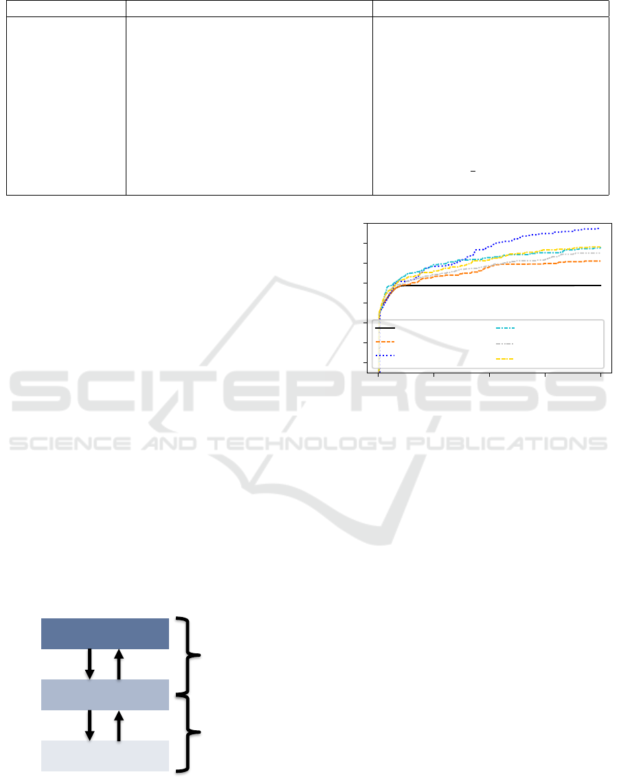
Table 3: Parameters and variants of CMA-ES with their value space for parameter tuning (de Nobel et al., 2021; van Rijn

et al., 2016).

Hyperparameter Description Space

λ Number of children derived from parents {4,6,..,20}

Ratio of parents selected from population {0.2,0.3,..,0.8}

Initial standard deviation {0.1,0.2,..,0.9}

Bound correction Correction if individual out of bounds {saturate, unif, COTN, toroidal, mirror}

Active update Covariance matrix update variation {on, off}

Elitism Strategy of the evolutionary algorithm {(µ, λ), (µ + λ)}

Mirrored sampling Mutations are the mirror image of another {on, off}

Orthogonal Orthogonal sampling {on, off}

Threshold Length threshold for mutation vectors {on, off}

Weights Weights for recombination {default, equal,

}

Restart Local restart of CMA-ES {off, IPOP, BIPOP}

used to calculate the utility of a CMA-ES conﬁgura-

tion during parameter tuning and ﬁnal validation.

To tune the parameters and select the best com-

bination of variants of CMA-ES, we use SMAC3

(Version 2.0.0) (Lindauer et al., 2022) as the meta-

algorithm. We use the default conﬁguration of SMAC

with an evaluation budget of 1 000 and perform three

full-parameter tuning runs on each tuning reference

and real-world problem.

5 TUNING RESULTS

We tune CMA-ES individually on each of the ﬁve

real-world problems yi and on the three most simi-

lar randomly generated artiﬁcial functions (Figure 5).

Then, the best derived conﬁguration from each pa-

rameter tuning run is validated on the real-world prob-

lem.

Figure 7 shows the Empirical Cumulative Distri-

bution Function for different CMA-ES conﬁgurations

on the real-world problem y1. We compared the re-

sults with the default CMA-ES conﬁguration and the

CMA-ES with IPOP enabled. By simply enabling

Meta-Algorithm

Algorithm

Tuning Reference

problem

solving

parameter

tuning

algorithm

quality

solution

quality

optimize

Figure 6: Solving the original problem and parameter tun-

ing as two different optimization problems.

0 500 1000 1500 2000

Evaluation budget

0.3

0.4

0.5

0.6

0.7

0.8

0.9

1.0

Fraction of runs + targets

default CMA-ES

IPOP CMA-ES

tuned on y1

tuned on AF

sim, 1

tuned on AF

sim, 2

tuned on AF

sim, 3

Figure 7: Empirical Cumulative Distribution Function for

different CMA-ES conﬁgurations on the real-world prob-

lem y1 that solved the problem within the budget given by

the x-axis.

IPOP, the performance increases with higher budgets.

The default CMA-ES stagnates because it does not

restart. Not surprisingly, the best performing con-

ﬁguration is the CMA-ES conﬁguration tuned to y1,

which almost always solves the optimization problem

within a budget of 2 000 evaluations. It is important

to note that conﬁgurations tuned to a similar artiﬁcial

function improve the performance compared not only

to the default conﬁguration but also to the CMA-ES

with IPOP enabled.

The parameter tuning and the validation vary

slightly due to random effects within the optimization

of SMAC and CMA-ES. Therefore, we perform three

parameter tuning runs on each problem and then val-

idate each of the derived conﬁgurations on the ﬁve

real-world problems yi with three individual valida-

tion runs. Figure 8 summarizes the results as the aver-

age of the three validation runs. Not surprisingly, the

IPOP CMA-ES always outperforms the pure default

conﬁguration of the CMA-ES without restart. The

parameter conﬁguration tuned to a real-world prob-

Real-World Optimization Benchmark from Vehicle Dynamics: Speciﬁcation of Problems in 2D and Methodology for Transferring

(Meta-)Optimized Algorithm Parameters

on y1 on y2 on y3 on y4 on y5

default

IPOP

tuned on y1

tuned on y2

tuned on y3

tuned on y4

tuned on y5

tuned on AF

sim, 1

tuned on AF

sim, 2

tuned on AF

sim, 3

tuned on BBOB

sim

tuned on Sphere

0.3 0.31 0.41 0.27 0.4

0.24 0.17 0.31 0.12 0.35

0.15 0.16 0.38 0.35 0.26

0.2 0.11 0.31 0.25 0.29

0.24 0.16 0.28 0.12 0.35

0.26 0.17 0.31 0.094 0.37

0.18 0.15 0.44 0.39 0.15

0.19 0.11 0.38 0.14 0.3

0.23 0.19 0.35 0.11 0.33

0.19 0.13 0.39 0.2 0.34

0.26 0.17 0.32 0.2 0.33

0.26 0.2 0.36 0.2 0.35

Figure 8: Utility (1 − AUC) of the default and IPOP CMA-

ES conﬁguration and the CMA-ES conﬁgurations tuned to

different functions (y-axis) when validating them on the ﬁve

real-world problems yi (x-axis). The smaller the value, the

better is the performance of the CMA-ES conﬁguration.

lem always performs best when validated again on the

same real-world problem.

In agreement with the similarity between two

problems (Figure 4), transferring CMA-ES conﬁgu-

rations tuned to one of the similar real-world prob-

lems y1 to y2 and transferring them to the other does

indeed improve performance. Transferring the more

dissimilar real-world problems y4 to y5 and vice versa

does not improve performance compared to the IPOP

CMA-ES.

CMA-ES conﬁgurations tuned on similar artiﬁ-

cial functions (AF) can almost always beat or com-

pete with the IPOP CMA-ES. Thus, tuning on similar

functions improves the performance on the original

optimization problem. Only for y3, IPOP CMA-ES is

always better than the CMA-ES conﬁgurations tuned

on the similar artiﬁcial functions.

The second most similar artiﬁcial function AF

sim,2

is the same function for y1 and y2 (Figure 5) and

therefore we get the same three tuned conﬁgurations.

The performance of these three tuned conﬁgurations

on AF

sim,2

is comparatively worse than the conﬁgura-

tions tuned to AF

sim,1

and AF

sim,3

when validated on

y1 and y2. The reason for this is the second parameter

tuning run, where the obtained best conﬁguration of

CMA-ES has no restart variant enabled. This leads to

the average poor performance of AF

sim,2

. Thus, restart

is not necessary for every function, even if this func-

tion is multimodal and very similar in terms of ELA

characteristics. In the future, to obtain a more robust

tuned conﬁguration of CMA-ES, the parameter tun-

ing of CMA-ES should be performed on more than

one similar artiﬁcial function.

The comparison with the most similar BBOB

function shows that tuning on the more similar artiﬁ-

cial functions leads to better results. Thus, generating

artiﬁcial functions as new tuning references instead of

selecting a similar BBOB function is recommended

and worth the effort to improve the performance of

CMA-ES.

Finally, tuning on the Sphere function also im-

proves the performance of CMA-ES compared to the

default conﬁguration of CMA-ES and also competes

with the IPOP CMAES. Tuning CMA-ES even on

a dissimilar function can improve the performance.

This conﬁrms the results from (Thomaser et al.,

2023b).

In summary, our results show that tuning improves

the performance of CMA-ES. Moreover, the more

similar two optimization problems are in terms of

ELA features, the better the performance when the

tuned conﬁguration of CMA-ES is transferred to the

other optimization problem.

6 CONCLUSION

In this paper, we compared CMA-ES conﬁgurations

tuned to ﬁve different real-world 2D vehicle dynam-

ics problems and compared the performance to CMA-

ES conﬁgurations tuned to other functions, referred

to as tuning references. We used Exploratory Land-

scape Analysis to quantify the similarity between two

optimization problems and to select the most similar

optimization problems from approximately 1000000

randomly generated artiﬁcial functions. The visual

appearance of the most similar artiﬁcial functions is

very similar to the original real-world problems.

Moreover, the CMA-ES conﬁguration tuned to

the similar artiﬁcial functions improved the perfor-

mance on the real-world problems compared to the

default CMA-ES conﬁguration, IPOP CMA-ES, and

also to CMA-ES conﬁgurations tuned to BBOB func-

tions. This encourages further pursuit of the approach

of transferring algorithm parameters tuned to similar

problems.

Future research should investigate whether the ad-

ditional computational effort for computing the ELA

features and tuning the parameters is justiﬁed. An-

other topic of future research is to investigate whether

the parameter tuning on several similar functions can

increase the robustness of the CMA-ES conﬁguration

when transferred to the original optimization prob-

lem.

ACKNOWLEDGEMENTS

This paper was written as part of the project newAIDE

under the consortium leadership of BMW AG with

the partners Altair Engineering GmbH, divis intelli-

gent solutions GmbH, MSC Software GmbH, Techni-

cal University of Munich, TWT GmbH. The project is

ECTA 2023 - 15th International Conference on Evolutionary Computation Theory and Applications

supported by the Federal Ministry for Economic Af-

fairs and Climate Action (BMWK) on the basis of a

decision of the German Bundestag.

REFERENCES

Auger, A. and Hansen, N. (2005). A Restart CMA Evo-

lution Strategy With Increasing Population Size. In

Proceedings of the IEEE Congress on Evolutionary

Computation, volume 2, pages 1769–1776.

ack, T. (1994). Parallel Optimization of Evolutionary Al-

gorithms. In Goos, G., Hartmanis, J., Leeuwen, J.,

Davidor, Y., Schwefel, H.-P., and M

anner, R., editors,

Parallel Problem Solving from Nature — PPSN III,

volume 866 of Lecture Notes in Computer Science,

pages 418–427. Springer Berlin Heidelberg, Berlin,

Heidelberg.

ack, T., Foussette, C., and Krause, P. (2013). Contempo-

rary Evolution Strategies. Natural Computing Series.

Springer Berlin, Heidelberg, Berlin, Heidelberg, 1st

ed. edition.

de Nobel, J., Vermetten, D., Wang, H., Doerr, C., and B

ack,

T. (2021). Tuning as a Means of Assessing the Bene-

ﬁts of New Ideas in Interplay with Existing Algorith-

mic Modules. Technical report.

Eiben, A. E. and Smit, S. K. (2011). Parameter tuning for

conﬁguring and analyzing evolutionary algorithms.

Swarm and Evolutionary Computation, 1(1):19–31.

Fujii, G., Takahashi, M., and Akimoto, Y. (2018). CMA-

ES-based structural topology optimization using a

level set boundary expression-Application to optical

and carpet cloaks. Computer Methods in Applied Me-

chanics and Engineering, 332:624–643.

Grefenstette, J. (1986). Optimization of Control Parameters

for Genetic Algorithms. IEEE Transactions on Sys-

tems, Man, and Cybernetics, 16(1):122–128.

Hansen, N. (2009). Benchmarking a BI-Population CMA-

ES on the BBOB-2009 Function Testbed. In Pro-

ceedings of the 11th Annual Conference Compan-

ion on Genetic and Evolutionary Computation Con-

ference: Late Breaking Papers, ACM Conferences,

pages 2389–2396, New York, NY, USA. Association

for Computing Machinery.

Hansen, N. (2016). The CMA Evolution Strategy: A Tuto-

rial. Technical report.

Hansen, N., Finck, S., Ros, R., and Auger, A. (2009).

Real-Parameter Black-Box Optimization Benchmark-

ing 2009: Noiseless Functions Deﬁnitions. Technical

Report RR-6829, INRIA.

Hansen, N. and Ostermeier, A. (1996). Adapting Arbitrary

Normal Mutation Distributions in Evolution Strate-

gies: The Covariance Matrix Adaptation. In Proceed-

ings of the IEEE International Conference on Evolu-

tionary Computation, pages 312–317.

International Organization for Standardization (2007). ISO

21994:2007 - Passenger cars - Stopping distance

at straight-line braking with ABS - Open-loop test

method.

Jolliffe, I. T. (1986). Principal Component Analysis.

Springer eBook Collection Mathematics and Statis-

tics. Springer, New York, NY.

Kerschke, P., Preuss, M., Wessing, S., and Trautmann, H.

(2015). Detecting Funnel Structures by Means of Ex-

ploratory Landscape Analysis. In Proceedings of the

2015 Annual Conference on Genetic and Evolutionary

Computation, ACM Digital Library, pages 265–272,

New York, NY. Association for Computing Machin-

ery.

Kerschke, P., Preuss, M., Wessing, S., and Trautmann, H.

(2016). Low-Budget Exploratory Landscape Analysis

on Multiple Peaks Models. In Neumann, F., editor,

Proceedings of the Genetic and Evolutionary Compu-

tation Conference, ACM Digital Library, pages 229–

236, New York, NY, USA. Association for Computing

Machinery.

Kerschke, P. and Trautmann, H. (2019). Comprehen-

sive Feature-Based Landscape Analysis of Continu-

ous and Constrained Optimization Problems Using the

R-Package Flacco. In Bauer, N., Ickstadt, K., L

ubke,

K., Szepannek, G., Trautmann, H., and Vichi, M., edi-

tors, Applications in Statistical Computing, Studies in

Classiﬁcation, Data Analysis, and Knowledge Orga-

nization, pages 93–123. Springer.

Koch-D

ucker, H.-J. and Papert, U. (2014). Antilock brak-

ing system (ABS). In Reif, K., editor, Brakes, Brake

Control and Driver Assistance Systems, Bosch profes-

sional automotive information, pages 74–93. Springer

Vieweg, Wiesbaden.

Lindauer, M., Eggensperger, K., Feurer, M., Biedenkapp,

A., Deng, D., Benjamins, C., Ruhkopf, T., Sass,

R., and Hutter, F. (2022). SMAC3: A Versatile

Bayesian Optimization Package for Hyperparameter

Optimization. Journal of Machine Learning Research,

23(54):1–9.

Long, F. X., van Stein, B., Frenzel, M., Krause, P., Gitterle,

M., and B

ack, T. (2022). Learning the Characteris-

tics of Engineering Optimization Problems with Ap-

plications in Automotive Crash. In Proceedings of the

Genetic and Evolutionary Computation Conference,

GECCO ’22, New York, NY, USA. Association for

Computing Machinery.

Loshchilov, I. and Hutter, F. (2016). CMA-ES for Hyperpa-

rameter Optimization of Deep Neural Networks.

Lunacek, M. and Whitley, D. (2006). The Dispersion Met-

ric and the CMA Evolution Strategy. In Proceedings

of the 8th Annual Conference on Genetic and Evolu-

tionary Computation, page 477. Association for Com-

puting Machinery.

Mersmann, O., Bischl, B., Trautmann, H., Preuss, M.,

Weihs, C., and Rudolph, G. (2011). Exploratory Land-

scape Analysis. In Lanzi, P. L., editor, Proceedings of

the 13th Annual Conference on Genetic and Evolu-

tionary Computation, ACM Conferences, pages 829–

836, New York, NY, USA. ACM.

Mersmann, O., Preuss, M., and Trautmann, H. (2010).

Benchmarking Evolutionary Algorithms: Towards

Exploratory Landscape Analysis. In Schaefer, R.,

Cotta, C., Kołodziej, J., and Rudolph, G., editors, Par-

allel Problem Solving from Nature, PPSN XI, Lecture

Real-World Optimization Benchmark from Vehicle Dynamics: Speciﬁcation of Problems in 2D and Methodology for Transferring

(Meta-)Optimized Algorithm Parameters

Notes in Computer Science, pages 73–82. Springer,

Berlin.

noz, M. A., Kirley, M., and Halgamuge, S. K. (2015).

Exploratory Landscape Analysis of Continuous Space

Optimization Problems Using Information Content.

IEEE Transactions on Evolutionary Computation,

19(1):74–87.

Owen, A. B. (1998). Scrambling Sobol’ and Niederreiter–

Xing Points. Journal of Complexity, 14(4):466–489.

Pacejka, H. B. and Bakker, E. (1992). THE MAGIC FOR-

MULA TYRE MODEL. Vehicle System Dynamics,

21(sup001):1–18.

Prager, R. P. (2023). pﬂacco: The R-package ﬂacco in na-

tive Python code. https://github.com/Reiyan/pﬂacco.

Preuss, M. (2012). Improved Topological Niching for Real-

Valued Global Optimization. In Applications of Evo-

lutionary Computation, volume 7248 of Lecture Notes

in Computer Science, pages 386–395. Springer, Berlin

and Heidelberg.

Rice, J. R. (1976). The Algorithm Selection Problem. In

Rubinoff, M. and Yovits, M. C., editors, Advances in

Computers, volume 15, pages 65–118. Elsevier Sci-

ence & Technology, Saint Louis.

Siemens Digital Industries Software (2020). Tire Sim-

ulation & Testing. https://www.plm.automation.

siemens.com/global/en/products/simulation-test/

tire-simulation-testing.html.

Skvorc, U., Eftimov, T., and Koro

sec, P. (2020). Under-

standing the problem space in single-objective numer-

ical optimization using exploratory landscape analy-

sis. Applied Soft Computing, 90.

Sobol’, I. M. (1967). On the distribution of points in a cube

and the approximate evaluation of integrals. Com-

putational Mathematics and Mathematical Physics,

7(4):86–112.

The MathWorks, Inc. (2015). Simulink. https://www.

mathworks.com/.

Thomaser, A., Vogt, M.-E., B

ack, T., and Kononova, A. V.

(2023a). Real-world Optimization Benchmark from

Vehicle Dynamics - Data and Code. https://doi.org/

10.5281/zenodo.8307853.

Thomaser, A., Vogt, M.-E., Kononova, A. V., and B

ack, T.

(2023b). Transfer of Multi-objectively Tuned CMA-

ES Parameters to a Vehicle Dynamics Problem. In

Emmerich, M., Deutz, A., Wang, H., Kononova, A. V.,

Naujoks, B., Li, K., Miettinen, K., and Yevseyeva, I.,

editors, Evolutionary Multi-Criterion Optimization,

pages 546–560, Cham. Springer Nature Switzerland.

Tian, Y., Peng, S., Zhang, X., Rodemann, T., Tan, K. C.,

and Jin, Y. (2020). A Recommender System for

Metaheuristic Algorithms for Continuous Optimiza-

tion Based on Deep Recurrent Neural Networks. IEEE

Transactions on Artiﬁcial Intelligence, 1(1):5–18.

van Rijn, S., Wang, H., van Leeuwen, M., and B

ack, T.

(2016). Evolving the structure of Evolution Strate-

gies. In 2016 IEEE Symposium Series on Computa-

tional Intelligence (SSCI), pages 1–8.

VIRES Simulationstechnologie GmbH (2020). Opencrg.

https://www.asam.net/standards/detail/opencrg/.

Ye, F., Doerr, C., Wang, H., and B

ack, T. (2022). Auto-

mated Conﬁguration of Genetic Algorithms by Tun-

ing for Anytime Performance. IEEE Transactions on

Evolutionary Computation, 26(6):1526–1538.

ECTA 2023 - 15th International Conference on Evolutionary Computation Theory and Applications