On Selecting Optimal Hyperparameters for Reinforcement Learning

Based Robotics Applications: A Practical Approach

Ignacio Fidalgo

, Guillermo Villate

, Alberto Tellaeche

and Juan Ignacio Vázquez

Computer Science, Electronics and Communication Technologies, University of Deusto,

Avenida de las Universidades 24, Bilbao, Spain

Keywords: Intelligent Robotics, Reinforcement Learning, Hyperparameters.

Abstract: Artificial intelligence (AI) is increasingly present in industrial applications and, in particular, in advanced

robotics, both industrial and mobile. The main problem of these type of applications is that they use complex

AI algorithms, in which it is necessary to establish numerous hyperparameters to achieve an effective training

of the same. In this research, we introduce a pioneering approach to reinforcement learning in the realm of

industrial robotics, specifically targeting the UR3 robot. By integrating advanced techniques like Deep Q-

Learning and Proximal Policy Optimization, we've crafted a unique motion planning framework. A standout

novelty lies in our application of the Optuna library for hyperparameter optimization, which, while not

necessarily enhancing the robot's end performance, significantly accelerates the convergence to the optimal

policy. This swift convergence, combined with our comprehensive analysis of hyperparameters, not only

streamlines the training process but also paves the way for efficient real-world robotic applications. Our work

represents a blend of theoretical insights and practical tools, offering a fresh perspective in the dynamic field

of robotics.

1 INTRODUCTION

Robotics in general and industrial robotics in

particular are one of the sectors that has undergone a

major technological revolution over the last decade.

With the parallel development of the digitalisation of

industrial processes (Savastano et al., 2019), the

explosion of the use of artificial intelligence in

industry (Peres et al., 2020), and the irruption of

collaborative robots (Sherwani et al., 2020), the way

of conceiving the use of robots in industry has

changed radically. In our opinion, two main new

trends can be identified when designing applications,

which are as follows:

 Flexibility and adaptability of robotic

applications to new conditions (new product,

change of operating conditions, etc.): In this case,

it is necessary to provide the robot with the

capacity to adapt to variations in the base process,

with the capacity to adjust parameters and

https://orcid.org/0000-0002-0951-2307

https://orcid.org/0009-0001-0783-7984

https://orcid.org/0000-0001-9236-1951

https://orcid.org/0000-0001-6385-5717

operation offline, or in simulation, being of vital

importance in order not to lose production time.

 Related to the previous point, current robotics

must adapt to operate in unstructured

environments by intensively applying artificial

intelligence for the automatic recognition of parts

even when there are occlusions, human-robot

collaboration, or for the autonomous learning of

new tasks using simulation environments.

In this context, to be able to design this kind of

robotic applications, it is necessary to make intensive

use of artificial intelligence, mainly using Deep

Learning (Goodfellow et al., n.d.) and Reinforcement

Learning techniques (Sutton & Barto, 2020). Both

techniques use in their different algorithms neural

networks of varying complexity depending on the

application, which require an effective adjustment of

hyperparameters for their correct training.

The work presented in 2013 (Kober et al., 2013)

already established a formal definition of the main

Fidalgo, I., Villate, G., Tellaeche, A. and Vázquez, J.

On Selecting Optimal Hyperparameters for Reinforcement Learning Based Robotics Applications: A Practical Approach.

DOI: 10.5220/0012158200003543

In Proceedings of the 20th International Conference on Informatics in Control, Automation and Robotics (ICINCO 2023) - Volume 1, pages 123-130

ISBN: 978-989-758-670-5; ISSN: 2184-2809

123

aspects of RL, and of the problems and advantages

arising from its application in a field as specific as

robotics.

More recently, the state of the art in

Reinforcement learning presents some interesting

works related to creating and obtaining robot

trajectories autonomously. For example, (Shahid et

al., n.d.) presents an RL-based approach, using

Proximal Policy Optimization (PPO), for the

manipulation of parts. In another work, Bézier curves

are used to obtain motion planning in autonomous

industrial robots (Scheiderer et al., 2019).

In another work presented in 2019, the authors

use Deep Reinforcement Learning to obtain the

planning of robot trajectories, focusing mainly on the

optimisation of reward functions (Xie et al., 2019).

Finally, another interesting work can be found in

(Bhuiyan et al., 2023), where the authors use distance

sensors to gather environmental measurements

necessary for the RL algorithm.

The use case presented in this paper is based on

the use of Reinforcement Learning for the

development of an optimal path planner for an

industrial robot UR3. Therefore, the following

sections of the paper will particularise the state of the

art and the problem definition to this type of machine

learning algorithms.

Finally, it is interesting to mention three papers,

published in the last three years, which address

problems similar to the use case presented in this

research work, but which do not use optimisation

techniques for the configuration of the best parameter

values in the algorithm used.

In (Ha et al., 2020) they use a multi-agent

reinforcement learning algorithm, using a soft actor

critic (SAC) algorithm with considerable internal

complexity. In a second paper (Li et al., 2022), they

also use an algorithm based on the actor-critic

scheme, automatically adjusting and limiting entropy.

Last but not least, in (Zhou et al., 2021) they use

what has been defined as residual reinforcement

learning. In all three works, the aim is to develop a

motion planner for robotics, and the approach

followed has been to use RL with more or less

complex algorithms.

In our research work, the aim is to obtain similar

performance to the aforementioned works, but using

a standard algorithm, such as PPO, and focusing the

effort on the optimisation of the parameters of this

algorithm.

2 REINFORCEMENT LEARNING

ALGORITHMS AND

HYPERPARAMETERS

Reinforcement Learning (RL) algorithms are a third

group of algorithms in the machine learning branch,

along with supervised and unsupervised learning

(clustering). Unlike these two more common groups

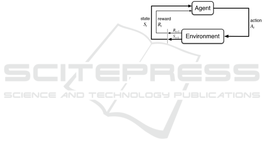
of algorithms, RL algorithms learn by trial and error.

The agent to be trained interacts with the environment

by executing actions and subsequently receives a

reward signal, as well as observations (states) about

the environment. This process is sequential and time-

dependent. A schematic of how this works can be

seen in Figure 1.

Figure 1: Schema of a RL algorithm (Shweta Bhatt, n.d.)

For a process to be solved by RL techniques, it is

necessary that the process follows a Markov decision

process (MDP), as stated in (Sutton & Barto, 2020).

A MDP is a Markov process in which the

environment provides a reward and allows decisions

to be taken. Mathematically, a MDP is a tuple

〈

𝑆,𝐴,𝑃,𝑅,𝛾

〉

where:

 S is a finite set or continuous value for states.

 A is a finite set or continuous value for

actions

 P is a state transition probability matrix

𝑃







=𝑃𝑟𝑜𝑏



𝑆



=𝑠



| 𝑆



=𝑠,𝐴





(1)

 R is the reward function

𝑅





=𝐸𝑥𝑝𝑒𝑐𝑡



𝑅



| 𝑆



=𝑠,𝐴





(2)

 γ is the discount factor 𝛾 𝜖



0,1



The main characteristic of this type of

environments is that for its learning, it depends only

on the current state of the problem, ignoring its

history or previous states. The objective is to obtain

the maximum reward possible for the episode, with

means to optimize actions in the problem given the

current state. This fact is defined by Bellman's

equation of optimality for the action-value function

(Lapan, 2018; Sutton & Barto, 2020)

Given the action-value function:

ICINCO 2023 - 20th International Conference on Informatics in Control, Automation and Robotics

124

𝑞



(

𝑠,𝑎

)

=𝑅





𝛾𝑃













𝜋

(

𝑎



𝑠



)







𝑞



(𝑠



,𝑎′)

(3)

The Bellman´s equation of optimality for the

action value function is:

𝑞

∗

(

𝑠,𝑎

)

= 𝑚𝑎𝑥



𝑞



(𝑠,𝑎) (4)

Where π represents the optimal policy, the

optimal behavioural function for the agent to solve

the environment.

Many of the RL environments to be solved

present continuous observation spaces of the

environment, i.e., the different observable states of

the environment take infinite continuous values

bounded between a maximum and minimum value.

To solve this problem, current algorithms use neural

networks to obtain the non-linear functions of the

policy and the value of the states. Two of the most

widely used algorithms that use this approach are

Deep Q-Learning (DQN) (Mnih et al., 2013) and PPO

(Schulman et al., 2017). Detailed technical

implementations can be found in the references cited

for each of these algorithms.

2.1 The Importance of

Hyperparameters

The following table presents the implementation

steps of the DQN algorithm:

Table 1: DQN algorithm implementation (Lapan, 2018).

Initialize parameters for Q(s,a) and Q^(s,a) with

random weights, ε=1.0 and empty the replay

buffer with N samples

With prob. Ε, select a random action a, otherwise

a= 𝑎𝑟𝑔𝑚𝑎𝑥



𝑄





Execute action a in the environment and observe

the reward r and the next state s’

4. Store transitions (s,a,r,s’) in the replay buffer

Sample a random minibatch of transitions from

the replay buffer

For every transition in the buffer, calculate target

y=r if the episode has ended at this step or 𝑦=

𝑟+𝛾𝑚𝑎𝑥



𝑄^(𝑠



,𝑎′) otherwise

7. Calculate loss 𝐿=(𝑄





−𝑦)



Update Q(s,a) using the SGD algorithm (Bottou,

1991) minimizing the loss in respect to model

parameters

Every M steps, copy network weights from Q(s,a)

to Q^(s,a)

10. Repeat from step 2 until convergence

As can be seen in table 1, the correct training and

operation of the algorithm depends on numerous

hyperparameters, some relating to the DQN algorithm

itself and others relating to the neural network used to

model the value function in this case. In our

experience, the hyperparameters that most influence

the learning of this algorithm are:

 Policy: Neural network architecture for

estimating the problem value function.

 Learning rate: The learning rate set for

policy training.

 Buffer size: size of the replay buffer to

obtain an initial uncorrelated dataset for

policy training.

 Batch size - Minibatch size for each gradient

update of the policy.

 gamma: Discount factor to weight the

importance of future states.

 Train frequency - Update frequency of the

neural network model of the policy.

 Exploration fraction (ε): Exploration factor

for moving from exploration to exploitation

of results in the solution of the problem.

 Exploration initial eps: Initial value of

exploration fraction.

 Exploration final eps: Final value of the

exploration fraction.

In the case of the PPO algorithm, rooted in the

actor-critic model, offers a structured approach to

reinforcement learning, ensuring effective training

and robust performance. A closer examination of its

design reveals the intricate interplay of various

hyperparameters, each contributing uniquely to the

algorithm's efficacy.

The Policy defines the neural network

architectures for both estimating the problem's value

function (critic) and the policy function (actor). Its

design and complexity can significantly influence the

algorithm's ability to generalize and learn from the

environment.

The Learning Rate is pivotal in determining how

quickly the algorithm updates its knowledge. A high

learning rate might lead to rapid convergence but

risks overshooting the optimal solution, while a low

rate ensures more stable learning at the expense of

longer training times.

The number of steps to execute per environment

update influence the granularity of learning and the

responsiveness of the model to changes in the

environment.

Batch Size determines the number of experiences

used in each update, striking a balance between

computational efficiency and gradient accuracy.

On Selecting Optimal Hyperparameters for Reinforcement Learning Based Robotics Applications: A Practical Approach

125

The Gamma discount factor emphasizes the

importance of future rewards. A value closer to 1

gives more weight to long-term rewards, while a

lower value prioritizes immediate rewards.

The N Epochs represents the number of iterations

when optimizing the loss function, determining the

depth of refinement for each batch of experiences.

Lastly, the Clip Range and Clip Range vf ensure

that the updates to the policy and value functions

remain bounded. These parameters prevent drastic

changes that could destabilize learning by ensuring

that the policy doesn't change too much in a single

update.

Figure 2: Different rewards and problem solutions obtained

depending on hyperparameters.

In essence, the choice and tuning of these

hyperparameters are not mere technicalities but are

central to the algorithm's success. Their optimal

values can vary based on the specific problem and

environment, underscoring the importance of

systematic experimentation and tuning.

Figure 2 shows the difference in training

efficiency of a simple problem, in this case the

CartPole problem available in the Gymnasium

library (Gymnasium: A Standard API for

Reinforcement Learning, n.d.)., using DQN.

Depending on the training hyperparameters

established the reward evolution of the problem,

differs.

3 PROBLEM DESCRIPTION

The goal of the proposed research is to develop a

motion planner using RL techniques, enabling a UR3

robot to accurately position its tool anywhere within

the workspace, maintaining the correct orientation.

Following this objective, the motion planner's

design becomes paramount. It must address the

nuanced problem of determining a sequence of valid

configurations that guide the UR3 robot from its

current position to the desired location. In this

specific context, the challenge isn't about navigating

around external obstacles, but rather ensuring that the

robot avoids collisions with itself and the floor. The

primary input to the motion planner is the robot's

current configuration and the desired goal position

and orientation.

Additionally, information about the robot's

structure and the floor's geometry is essential to avoid

self and floor collisions. The output from the motion

planner is a sequence of configurations that the robot

should adopt to reach the desired goal without any

collisions. In this scenario, the motion planner,

underpinned by RL techniques, aims to navigate the

robot's own structure and the immediate environment,

ensuring smooth and safe movement while

maintaining the tool's precise orientation.

The following figures shows in detail the

simulation environment used for this problem, based

on the physics engine PyBullet (Coumans, n.d.).

This problem is defined with continuous

observation space of dimension 14 according to the

equation 5:

𝑂𝑏𝑠𝑆𝑝𝑎𝑐𝑒 =

(

𝑥,𝑦,𝑧,𝑜𝑋,𝑜𝑌,𝑜𝑍,𝑜𝑊,𝜃



,𝜃



,𝜃



,𝜃



,𝜃



,𝜃



,𝑐𝑜𝑙𝑙𝑖𝑠𝑖𝑜𝑛

)

(5)

Where x, y, z are the cartesian distances to the

target point, oX, oY, oZ, oW are the orientation

differences to the desired orientation at the target

point given in quaternions, θ

are the values of the

angles of the different joints and finally a collision

flag is included, in order to obtain valid trajectories.

Figure 3: Simulation environment (view 1).

The action space has 6 dimensions. Each of these

values are bounded between -1 and 1, using these

results per joint as a multiplicative factor of the angle

of movement per maximum step established for each

one of the joints (θ

max

). according to the equation 6:

𝐴

𝑐𝑡𝑆𝑝𝑎𝑐𝑒

=𝜃



(

𝛼



,𝛼



,𝛼



,𝛼



,𝛼



,𝛼



)

| 𝛼



𝜖



−1,1



(6)

ICINCO 2023 - 20th International Conference on Informatics in Control, Automation and Robotics

126

In the context of the UR3 robot's operation, these

values need to be translated into meaningful

commands. To achieve this, the float values are

scaled to match the permissible angle range of each

of the robot's joints. By doing so, each normalized

action value is converted into a joint angle between

-2π and 2π, allowing for direct command execution

by the robot.

The reward for this problem is defined using the

following algorithm:

Algorithm 1: Reward function.

Data: ObsSpace; p1, q1, collision

EnvironmentInf: p2, q2, prev_dist

if collision == 1 then

return -250

d (p1, p2) = euclidean_distance (p1, p2)

d (q1, q2) = 1−

〈

𝑞1,𝑞2

〉



if d (p1, p2) < 0.01 & d (q1, q2) < 0.01 then

return 300

∆d = prev_dist – d(p1, p2) -d(q1, q2)

prev_dist = d(p1, p2) + d(q1, q2)

return ∆d * 100

As the training progresses and the motion planner

refines its policy, these joint angle commands

collectively form a coherent and valid trajectory.

Once the training is complete, this trajectory

ensures that the robot can smoothly and accurately

move its tool to the desired position and orientation

within the workspace.

Figure 4: Simulation environment (view 2).

4 PARAMETER OPTIMIZATION

As explained in previous sections, the optimisation of

the different hyperparameters of the RL algorithm to

be used for the solution of a problem is fundamental

for the optimal learning of the algorithm, thus making

it possible to solve the problem in an optimal number

of steps.

This consideration becomes even more critical in

complex problems where the algorithm's learning

time is substantial. For the hyperparameter

optimization in the problem described, we utilized the

Optuna library (Akiba et al., 2019).

For the optimisation of hyperparameters in the

problem described above, the Optuna library (Akiba

et al., 2019) has been used. This Python library is used

for general mathematical optimisation problems,

where objective functions can be defined to be

maximised or minimised, depending on the problem.

In the case of RL problems such as the one we are

dealing with, the way to optimise parameters

effectively is to train the RL algorithm within this

objective function.

At its core, Optuna requires the definition of an

objective function, which serves as the benchmark

against which the performance of different

hyperparameter configurations is evaluated. The

process begins with Optuna suggesting feasible

values for each hyperparameter based on predefined

search spaces. For this purpose, the following search

spaces are used:

• Policy: More precisely, the number of

neurons per layer. Categorical value of

[32, 64, 128, 256] neurons.

• Learning rate of the policy and critic

networks. Floating number range [ 3



,110



• Batch size for network training. Integer

number range [1, 24].

• Discount factor (gamma). Floating

number range [0.9,0.99]

• Number of epochs. Integer number

range [3, 20].

• Clip range. Floating number range

[0.1,0.3].

With these values, an RL training session is

initiated using the suggested hyperparameters. To

ensure efficiency and relevance, the number of

training steps is benchmarked against the baseline,

providing a constraint that guides the optimization

process. For every RL training session, the final mean

reward of the policy is used as the Optune objective

output.

As the iterations progress, Optuna intelligently

adjusts its suggestions based on the objective function

output of previous configurations, aiming to find the

optimal set of hyperparameters that maximize the

objective function’s output. This iterative and

adaptive approach ensures that the RL model is

trained with the most suitable hyperparameters,

enhancing its performance and reducing the overall

training time.

On Selecting Optimal Hyperparameters for Reinforcement Learning Based Robotics Applications: A Practical Approach

127

5 OBTAINED RESULTS

Hyperparameter optimisation using Optuna has been

used to optimise the learning process and maximise

the reward obtained in the RL problem presented in

section 3 of the paper.

According to the literature and to the state of the

art, the PPO algorithm has been selected for the

solution of this problem.

A total of 100 parameter optimisation iterations

have been performed, training each of these iterations

for 150,000 steps.

This number of steps has been established by

observing the convergence of the reward for this

problem taking the default parameters established for

the PPO algorithm.

Of the 100 hyperparameter optimisation tests

performed, trials 47 and 70 are the best performers

according to the reward plots obtained for training.

Table 2 shows the PPO baseline parameters and

the optimum parameters calculated in the 47 and 70

trials.

Table 2: Optimization parameters obtained with Optuna

Paramete

PPO

aseline

Trial 47

Optuna

Trial 70

tuna

etwork

size

64 neuron

per layer,

two la

ers

64 neuron

per layer,

two la

ers

64 neuron

per layer,

two la

ers

Learning

rate

0.0003 553.52e-

0.00076

. Steps 2048 300 300

Batch size 64 12 12

. Epochs 10 11 8

Gamma 0.99 0.9 0.9

Clip

Range

0.2 0.2 0.2

As can be seen in the table above, the optimised

parameters in iterations 47 and 70 have similar values

for almost all parameters, and in turn differ quite a lot

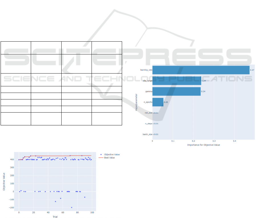
Figure 5: Optimization history (Optuna).

from the default parameters provided by the PPO

algorithm in the Stable Baselines 3 reinforcement

learning library (Raffin et al., 2021).

In the following images you can see the

optimisation history carried out by Optuna (figure 5)

and the relative importance of each of the

hyperparameters in the final result of the optimisation

(figure 6).

Finally, to demonstrate the effectiveness of

hyperparameter optimisation in RL problems, this

section finally presents the reward and episode length

plots for the problem proposed in section 3, both for

the default PPO parameters (baseline of the problem)

and for the optimal parameters obtained and

previously presented in table 2.

On the one hand, the reward plot shows the

learning convergence speed of the problem,

estimating it when it is taken to the maximum value

of reward and this is kept constant. It also allows us

to observe the maximum reward obtained, also

showing the effectiveness of the agent in solving the

problem.

The graph illustrating the average episode lengths

for each set of chosen hyperparameters further

underscores the effectiveness of our solution

approach. The shorter the length of the episodes, the

fewer steps the agent needs to solve the problem, so

it is a more effective agent.

Figure 6: Hyperparameter relative importance to optimize

the final objective value.

Figure 7 shows the average reward obtained

during the training process, the values obtained by the

baseline PPO are represented in the blue graph, while

Optuna iteration 47 is shown in green, and 70 in red.

As shown, the baseline PPO needs 125k steps for

the convergence of the training, while the other two

options reach the optimal result in 50k, i.e., the

learning capacity of the problem is improved, taking

3 times less time.

ICINCO 2023 - 20th International Conference on Informatics in Control, Automation and Robotics

128

Figure 7: Reward graph for PPO baseline (orange),

Optuna iteration 47 (grey) and Optuna iteration 70 (blue).

Moreover, figure 8 shows the average episode

lengths during training for these three configurations.

As is logical after observing the previous reward plot,

the average episode lengths for the Optuna

configurations are much shorter than those obtained

by the baseline PPO, showing a superior effectiveness

in training the RL agent.

Figure 8: Episode length for PPO baseline (orange),

Optuna iteration 47 (grey) and Optuna iteration 70 (blue).

While the performance of the robot remains

relatively consistent as it converges to the optimal

policy, a notable advantage emerges in the speed of

this convergence. The research indicates that, even if

the end performance metrics of the robot do not show

substantial improvement, the time taken to reach this

optimal policy is significantly reduced. This faster

convergence can lead to more efficient training

processes and quicker deployment of robotic

solutions in real-world scenarios, emphasizing the

importance of optimizing the learning process even if

the end performance remains unchanged.

6 CONCLUSIONS AND FUTURE

WORK

In this research work, a practical study and parameter

optimisation method has been carried out on a

reinforcement learning algorithm, PPO, used to

control a UR3 industrial robot.

It has been shown that the correct choice of

optimal hyperparameters for the resolution of a

problem of this type is fundamental to reach a fast

convergence and to obtain an effective policy in the

shortest possible training time of the algorithm.

This last point, the necessary training time, is of

special importance in problems based on RL

techniques, since it grows exponentially with the

complexity of the problem, being usual to need to

execute millions of training steps for any typical

problem in the field of robotics.

For this reason, the method is of particular value

for the efficiency of training this type of algorithms.

As future work, it would be necessary to carry out

a scientific study of the influence that each of the

hyperparameters has on the convergence of a given

reinforcement learning algorithm.

In this first work in this respect, the parameters

have been selected empirically, observing which ones

were particularly relevant in the learning stage of the

algorithm. Once those considered most relevant have

been selected, they have been optimised using the

Optuna library.

An important advance to this procedure would be

scientific justification of the choice of

hyperparameters to be optimised, which is considered

the missing step for a complete optimisation process

of the training of RL algorithms.

ACKNOWLEDGEMENTS

This research was carried out within the project

ACROBA which has received funding from the

European Union’s Horizon 2020 research and

innovation programme, under grant agreement No

101017284.

REFERENCES

Akiba, T., Sano, S., Yanase, T., Ohta, T., & Koyama, M.

(2019). Optuna: A Next-generation Hyperparameter

Optimization Framework. Proceedings of the ACM

SIGKDD International Conference on Knowledge

Discovery and Data Mining, 2623–2631.

https://doi.org/10.1145/3292500.3330701

Bhuiyan, T., Kästner, L., Hu, Y., Kutschank, B., &

Lambrecht, J. (2023). Deep-Reinforcement-Learning-

based Path Planning for Industrial Robots using

Distance Sensors as Observation. http://arxiv.org/

abs/2301.05980

On Selecting Optimal Hyperparameters for Reinforcement Learning Based Robotics Applications: A Practical Approach

129

Bottou, L. (1991). Stochastic Gradient Learning in Neural

Networks.

Coumans, E. (n.d.). PyBullet Physics Engine.

Https://Pybullet.Org/Wordpress/.

Goodfellow, I., Bengio, Y., & Courville, A. (n.d.). Deep

Learning.

Gymnasium: A standard API for reinforcement learning.

(n.d.). Https://Gymnasium.Farama.Org/.

Ha, H., Xu, J., & Song, S. (2020). Learning a Decentralized

Multi-arm Motion Planner. http://arxiv.org/abs/2011.

02608

Kober, J., Bagnell, J. A., & Peters, J. (2013). Reinforcement

learning in robotics: A survey. International Journal of

Robotics Research, 32(11), 1238–1274.

https://doi.org/10.1177/0278364913495721

Lapan, M. (2018). Deep Reinforcement Learning Hands-

On.

Li, X., Liu, H., & Dong, M. (2022). A General Framework

of Motion Planning for Redundant Robot Manipulator

Based on Deep Reinforcement Learning. IEEE

Transactions on Industrial Informatics, 18(8), 5253–

5263. https://doi.org/10.1109/TII.2021.3125447

Mnih, V., Kavukcuoglu, K., Silver, D., Graves, A.,

Antonoglou, I., Wierstra, D., & Riedmiller, M. (2013).

Playing Atari with Deep Reinforcement Learning.

http://arxiv.org/abs/1312.5602

Peres, R. S., Jia, X., Lee, J., Sun, K., Colombo, A. W., &

Barata, J. (2020). Industrial Artificial Intelligence in

Industry 4.0 -Systematic Review, Challenges and

Outlook. IEEE Access. https://doi.org/10.1109/

ACCESS.2020.3042874

Raffin, A., Hill, A., Gleave, A., Kanervisto, A., Ernestus,

M., & Dormann, N. (2021). Stable-Baselines3: Reliable

Reinforcement Learning Implementations. In Journal

of Machine Learning Research (Vol. 22).

https://github.com/DLR-RM/stable-baselines3.

Savastano, M., Amendola, C., Bellini, F., & D’Ascenzo, F.

(2019). Contextual impacts on industrial processes

brought by the digital transformation of manufacturing:

A systematic review. Sustainability (Switzerland),

11(3). https://doi.org/10.3390/su11030891

Scheiderer, C., Thun, T., & Meisen, T. (2019). Bézier curve

based continuous and smooth motion planning for self-

learning industrial robots. Procedia Manufacturing, 38,

423–430. https://doi.org/10.1016/j.promfg.2020.01.

054

Schulman, J., Wolski, F., Dhariwal, P., Radford, A., &

Klimov, O. (2017). Proximal Policy Optimization

Algorithms. http://arxiv.org/abs/1707.06347

Shahid, A. A., Roveda, L., Piga, D., & Braghin, F. (n.d.).

Continuous Control Actions Learning and Adaptation

for Robotic Manipulation through Reinforcement

Learning.

Sherwani, F., Asad, M. M., & Ibrahim, B. S. K. K. (2020).

Collaborative Robots and Industrial Revolution 4.0 (IR

4.0). https://www.mirai-lab.co.jp/

Shweta Bhatt. (n.d.). Reinforcement Learning 101: Learn

the essentials of Reinforcement Learning!

Https://Towardsdatascience.Com/Reinforcement-

Learning-101-E24b50e1d292.

Sutton, R. S., & Barto, A. G. (2020). Reinforcement

learning : an introduction (2nd Edition). The MIT Press.

Xie, J., Shao, Z., Li, Y., Guan, Y., & Tan, J. (2019). Deep

Reinforcement Learning with Optimized Reward

Functions for Robotic Trajectory Planning. IEEE

Access, 7, 105669–105679. https://doi.org/10.1109/

ACCESS.2019.2932257

Zhou, D., Jia, R., Yao, H., & Xie, M. (2021). Robotic Arm

Motion Planning Based on Residual Reinforcement

Learning. 2021 13th International Conference on

Computer and Automation Engineering, ICCAE 2021,

89–94. https://doi.org/10.1109/ICCAE51876.2021.

9426160.

ICINCO 2023 - 20th International Conference on Informatics in Control, Automation and Robotics

130