
Bayesian Hierarchical Modelling of Basketball Team Performance:
An NBA Regular Season Case Study
Paul Attard
a
, David Suda
b
and Fiona Sammut
c
Department of Statistics and Operations Research, University of Malta, Msida, MSD 2080, Malta
Keywords: Bayesian Hierarchical Models, Basketball, Scoring Intensity Models, Winning Probability Models.
Abstract: The main goal of this study is to propose two Bayesian hierarchical modelling approaches using basketball
game data from the 2008/2009 NBA regular season. The aim of the first approach is to estimate the results of
each match during the season. This is done by considering each scoring method in basketball separately, that
is, free throws, 2-point shots and 3-point shots, and estimating the offensive and defensive ability with respect
to each scoring method for each team. These attributes are then used to produce a final score for each match.
We attempt both the Poisson and the negative binomial distribution to model the scoring propensities. Both
models are used to predict game outcomes and final standings, and since we find the negative binomial
approach to be considerably superior, we use it to determine overall attack and defense abilities of each time
for each scoring method. The second modelling approach, on the other hand, focuses on finding the probability
of the home team winning a particular match in the season. Due to MCMC convergence issues, this model is
represented by just one parameter representing overall strength for each team rather than two. When
comparing the winning probability approach with the scoring propensity approach, we find that the latter is
superior at predicting game outcomes, the former is superior at predicting final standings, while both are
comparable in predicting which teams will qualify to playoffs.
1 INTRODUCTION
The main objective of this paper is to propose a
Bayesian hierarchical approach to modelling
basketball scores, and consequently games outcomes,
in a league. While our focus will be on basketball,
literature on other sports will be referenced, and
required adjustments for the basketball application
shall be made. In the following, we shall first focus
on literature related to statistical modelling related to
basketball and Bayesian hierarchical modelling.
Next, we will provide the mathematical formulation
for the Bayesian hierarchical structure of the
proposed models, which are built with two basketball
game related applications in mind, related to
modelling the scoring intensity and the winning
probability. Finally, we will fit the different models
and compare results to determine which Bayesian
hierarchical models are the most suitable for game
prediction and standings prediction for the dataset
a
https://orcid.org/0009-0004-7647-3860
b
https://orcid.org/0000-0003-0106-7947
c
https://orcid.org/0000-0002-4605-9185
under study, which is the 2008/2009 NBA (National
Basketball Association) regular season. The scoring
intensity models shall also be used to measure the
teams’ attack and defense attributes.
2 LITERATURE REVIEW
In this section, we provide a literature review that
focuses on two aspects. The first is the use of
statistical analysis to model phenomena in the
basketball game, and the second is the use of
Bayesian modelling, and more specifically Bayesian
hierarchical modelling, in sports literature.
An early application of sports modelling to
basketball is the use of models which estimate the
probability that a specific team in the NCAA would
win the whole tournament (Carlin, 1996). External
information regarding the teams’ strengths along with
the point spreads available prior to the start of the
Attard, P., Suda, D. and Sammut, F.
Bayesian Hierarchical Modelling of Basketball Team Performance: An NBA Regular Season Case Study.
DOI: 10.5220/0012159100003587
In Proceedings of the 11th International Conference on Sport Sciences Research and Technology Support (icSPORTS 2023), pages 101-111
ISBN: 978-989-758-673-6; ISSN: 2184-3201
Copyright © 2023 by SCITEPRESS – Science and Technology Publications, Lda. Under CC license (CC BY-NC-ND 4.0)
101

tournament were used to improve the proposed
models. Another application is the use of a maximum
score estimator to predict final scores (Caudill, 2003).
This is an improvement to a probit model which
forms a relationship between a team’s seed and the
probability of them winning (Boulier and Stekler,
1999). Not only within the basketball context, the
idea that a team’s ability or strength is something
dynamic and can fluctuate throughout the course of a
season or a tournament is applied via an extension of
the Bradley–Terry model for paired comparison data,
to model the outcomes of sport events while allowing
for time varying abilities through the use of weighted
moving averages (Catellan et al., 2013). This was
applied to the 2009-2010 NBA regular season
(basketball) along with the 2008-2009 Italian Serie A
season (football). The use of player-tracking data at
every moment in a team’s possession of the ball to
produce a quantity called expected possession value
(EPV), has also been applied (Cervone et al., 2014).
EPV is an expectation of how many points the
attacking team is expected to score by the end of the
possession. This quantity was first introduced to
football where it was considered quite a revolutionary
new metric as it provides a team with data regarding
what would happen on an average basis if the team
was scheduled for an infinite number of matches.
Now, it is slowly making its way over to other sports
including basketball.
One early attempt of the use of Bayesian
modelling in sports is a Bayesian framework to the
bivariate Poisson distribution (Tsionas, 2001), which
was originally applied in a frequentist context in
football games (Karlis and Ntzoufras, 2000; Karlis
and Ntzoufras, 2003). The influential seminal paper
on the use of Bayesian hierarchical modelling in
sports, where each individual team’s number of goals
scored is assumed to follow a Poisson distribution, is
applied to the Italian Serie A championship
1991/1992 (Baio and Blangiardo, 2010). There have
also been other approaches on the use of Bayesian
hierarchical models to predict the outcome of tennis
matches (Ingram, 2019) and women’s volleyball
(Gabrio, 2020). In the former, a Bayesian hierarchical
model based on the binomial distribution is used to
model the serve-match, and in the latter, a Bernoulli-
based Bayesian hierarchical model is used to model
the probability of playing five sets, and the
probability of winning a match. To our knowledge,
the Bayesian hierarchical modelling approach has not
been applied to the basketball context. The Bayesian
hierarchical Poisson model (Baio and Blangiardo,
2010) shall serve as the basis for modelling scoring
intensity, and this shall be extended to the negative
binomial approach. Furthermore, the Bernouilli-
based Bayesian hierarchical modelling approach
applied to volleyball (Gabrio, 2020) shall serve as the
backbone for modelling the winning probability.
3 BAYESIAN HIERARCHICAL
MODELLING OF SCORING
INTENSITY
A noteworthy difference between the goals scored in
football and basketball is that, in football you have
one method of increasing the number of goals in a
match, which always increments by a single value for
each goal, while in basketball there are three different
ways to score and how one can increase their team’s
point tally. These different ways would be the free
throw (1 point), the two-point shot, and the three-
point shot. Due to this difference, it was felt necessary
that each scoring method should be modelled
separately and in the end, the totals would be summed
up according to their respective weight in order to
obtain the predicted final score. We first start by
defining the Bayesian hierarchical Poisson model
applied to basketball, and then move on to extending
this to the negative binomial case.
3.1 The Poisson Model
In this study, three Poisson models separately shall be
considered (free throws made, two point shots made
and three point shots made):
𝐹𝑇
| 𝜃
~ 𝑃𝑜𝑖𝑠𝑠𝑜𝑛(𝜃
)
𝑇𝑤𝑜𝑃𝑇
| 𝜃
~ 𝑃𝑜𝑖𝑠𝑠𝑜𝑛(𝜃
) (1)
𝑇ℎ𝑟𝑒𝑒𝑃𝑇
| 𝜃
~ 𝑃𝑜𝑖𝑠𝑠𝑜𝑛(𝜃
)
where 𝑔 represents the match index (in order of the
date and time they were played), 𝑗 represents whether
the team played at home or away (1 – home effect, 2
– away effect). 𝐹𝑇
, 𝑇𝑤𝑜𝑃𝑇
and 𝑇ℎ𝑟𝑒𝑒𝑃𝑇
represent the observed count for the free throws, two-
point shots and three-point shots made by team 𝑗 in
the g
th
match, respectively. 𝜃
, 𝜃
and
𝜃
represent the scoring intensity with
respect to free throws, two-point shots and
three-point
shots by team 𝑗 in the g
th
match, respectively. The
scoring intensity of the home and away team shall be
estimated by considering the attack and defense
ability for each team along with the home effect. The
models must also include an intercept common for
both scoring intensities due to the fact that basketball
icSPORTS 2023 - 11th International Conference on Sport Sciences Research and Technology Support
102

scores can take large values. These parameters were
again modelled using a log-linear random effect
model:
𝑙𝑜𝑔
𝜃
= 𝑎𝑡𝑡
()
+ 𝑑𝑒𝑓
()
+ 𝑐
+ ℎ𝑜𝑚𝑒
𝑙𝑜𝑔
𝜃
= 𝑎𝑡𝑡
()
+ 𝑑𝑒𝑓
()
+ 𝑐
(2)
where 𝑎𝑡𝑡
represents the attack intensity for team 𝑡
(which can take 30 different values for 30 different
teams) with respect to model 𝑀 (which can be FT,
2PT or 3PT). Similarly, 𝑑𝑒𝑓
represents the defense
intensity for team t with respect to model 𝑀. It is
important to notice that a high and low 𝑎𝑡𝑡 value
represents a good and bad attacking strength for a
team, respectively. On the contrary, a high and low
𝑑𝑒𝑓 value represents a bad and good defending
strength for a team, respectively. Also, ℎ(𝑔) and
𝑎(𝑔) represent the team index (all teams listed in
order alphabetically) for the home and away team in
match g, respectively. The ℎ𝑜𝑚𝑒
represents the
advantage (for each model 𝑀) for the home team due
to playing at their home court and due to a vast
majority of the fans supporting them. Finally, 𝑐
represents a common intercept for all teams under
model 𝑀. This intercept was imperative for the model
to work correctly, due to the nature of a basketball
match having high score numbers. Also, nowadays,
each scoring method can be found multiple times in
every single match implying that the mean for each
predicted scoring method value had to be shifted
away from zero, justifying the inclusion of the
intercept in this model.
A suitable prior distribution must be assigned to
each parameter. In order to put the focus on the data
at hand, the following flat prior distributions shall be
considered:
ℎ𝑜𝑚𝑒
~ 𝑁𝑜𝑟𝑚(0, 0.0001)
𝑐
~ 𝑁𝑜𝑟𝑚(0, 0.0001) (3)
similar to the model based on the Italian football
league (Baio and Blangiardo, 2010). The parameters
𝑎𝑡𝑡
and 𝑑𝑒𝑓
are further assigned two
interchangeable (common for home and away)
hyperparameters each, which in turn, are also
modelled independently using flat prior distributions
where 𝜇
/
are assumed to follow normal
distributions with mean 0 and precision 0.0001 while
𝜏
/
are assumed to follow gamma distributions
with shape and scale parameters both 0.01, i.e.
𝑎𝑡𝑡
~ 𝑁𝑜𝑟𝑚(𝜇
, 𝜏
)
𝑑𝑒𝑓
~ 𝑁𝑜𝑟𝑚(𝜇
, 𝜏
)
𝜇
~ 𝑁𝑜𝑟𝑚(0, 0.0001) (4)
𝜇
~ 𝑁𝑜𝑟𝑚(0, 0.0001)
𝜏
~ 𝐺𝑎𝑚𝑚𝑎
(
0.1, 0.1
)
𝜏
~ 𝐺𝑎𝑚𝑚𝑎(0.1, 0.1)
Also, we applied constraints to the parameters 𝑎𝑡𝑡
and 𝑑𝑒𝑓
for identifiability purposes.
∑
𝑎𝑡𝑡
=0 and
∑
𝑑𝑒𝑓
=0 (5)
Figure 1: DAG of the general case for the scoring intensity
models using the Poisson distribution.
Since the NBA consists of 30 teams, this means
that each model will be working with 30 different 𝑎𝑡𝑡
parameters and 30 different 𝑑𝑒𝑓 parameters for each
team along with one value each for the ℎ𝑜𝑚𝑒
parameter and the overall intercept 𝑐. Thus, in total
we are going to be handling 186 different parameters
which combined together will ultimately provide us
with the total expected points scored by the home and
away team. Naturally, this is calculated at the end by
considering the number of points provided by each
scoring method. i.e.,
𝑇𝑃
= 𝐹𝑇
+ 2∗𝑇𝑤𝑜𝑃𝑇
+3∗(𝑇ℎ𝑟𝑒𝑒𝑃𝑇
)
(6)
Letting 𝑀
represent the observed count for each
model ( 𝐹𝑇
, 𝑇𝑤𝑜𝑃𝑇
and 𝑇ℎ𝑟𝑒𝑒𝑃𝑇
) , we can
represent each hierarchical model graphically in a
similar manner. Figure 1 shows a graphical
representation of the hierarchical structure for the
Bayesian Hierarchical Modelling of Basketball Team Performance: An NBA Regular Season Case Study
103

general case using the Poisson scoring intensity
model.
3.2 The Negative Binomial Model
Although the Poisson setup could potentially be an
acceptable model for the basketball application, a
distribution which could turn out to be a better choice
in the case of basketball would the negative binomial
distribution. This is due to the larger flexibility thanks
to its second parameter. This flexibility should be able
to compensate for the nature of points in a basketball
match always taking a large value, far from 0.
Analogous to the Poisson formulation, under the
negative binomial setup, three separate models shall
also be considered:
𝐹𝑇
| 𝑙
, 𝑟
~ 𝑁𝑒𝑔𝐵𝑖𝑛(𝑙
, 𝑟
)
𝑇𝑤𝑜𝑃𝑇
| 𝑙
, 𝑟
~ 𝑁𝑒𝑔𝐵𝑖𝑛(𝑙
, 𝑟
)
𝑇ℎ𝑟𝑒𝑒𝑃𝑇
| 𝑙
, 𝑟
~ 𝑁𝑒𝑔𝐵𝑖𝑛(𝑙
, 𝑟
)
(7)
where once again, g represents the match time order
index, 𝑗 represents whether the team played at home
or away (1 – home, 2 – away). 𝐹𝑇
, 𝑇𝑤𝑜𝑃𝑇
and
𝑇ℎ𝑟𝑒𝑒𝑃𝑇
represent the observed count for the free
throws, two point shots and three points made by
team 𝑗 in the 𝑔
match, respectively.
Figure 2: DAG of the general case for the scoring intensity
models using the negative binomial distribution.
Differently to the Poisson setup, 𝑟
, 𝑟
and
𝑟
represent the stopping parameters with
respect to free throws, two point shots and
three point
shots by team 𝑗 in the 𝑔
match, respectively.
Moreover, 𝑙
, 𝑙
and 𝑙
represent
the success probability parameters with respect to free
throws, two point shots and three point shots by team
𝑗 in the 𝑔
match, respectively. These parameters
were once again modelled using a log-linear random
effect model:
𝑙𝑜𝑔
𝑟
= 𝑎𝑡𝑡
()
+ 𝑑𝑒𝑓
()
+ 𝑐
+ ℎ𝑜𝑚𝑒
𝑙𝑜𝑔
𝑟
= 𝑎𝑡𝑡
()
+ 𝑑𝑒𝑓
()
+ 𝑐
(8)
The parameters mentioned in (8) have the same
definitions as in (3) and (4), and the hyperparameters
are also similarly defined. The parameters 𝑙
were
assigned uniform distributions ranging from 0 to 1. It
is imperative that they take a value between 0 and 1
since they represent a success probability, i.e.,
𝑙
~ 𝑈𝑛𝑖𝑓(0,1). A graphical representation of the
hierarchical model for the general case (scoring
method 𝑀) using the negative binomial distribution,
can be seen in Figure 2. The total points scored are
also obtained as in (6).
Both the models in Section 3.1 and 3.2 are
estimated using Gibbs sampling, which is an MCMC
approach for simulating values from the desired
parameters. For the algorithm for Gibbs sampling in
the Bayesian hierarchical context, see e.g. (Gelman et
al., 2004). In the next section, we go through the
construction of the Bayesian hierarchical winning
probability model.
4 BAYESIAN HIERARCHICAL
MODELLING OF WINNING
PROBABILITY
For our approach with respect to basketball, a slightly
different procedure was taken albeit with similarities
to the setup in the Bernoulli-based Bayesian
hierarchical model on women’s volleyball (Gabrio,
2020). Firstly, the idea of sets is non-existent in
basketball (as opposed to volleyball) so that part of
the model in the mentioned paper is not considered.
Secondly, since the binary variable which needs to be
estimated depends directly on the number of points
scored by each team in a particular match, one cannot
include these same variables in the logit function in
the same way as in this paper. Originally, the option
was to use the same predictor variables as those
specified in the scoring intensity models, except for
the home advantage since the intercept parameter
sufficed. However, due to issues of convergence in
the Gibbs sampler, it was finally decided that each
icSPORTS 2023 - 11th International Conference on Sport Sciences Research and Technology Support
104

team is only represented with one parameter which
we shall refer to as the strength, rather than making a
distinction between attack and defense parameters.
The model which we will be using will be of the form:
𝑑
≔ 𝕀
𝑦
𝑦
~ 𝐵𝑒𝑟𝑛𝑜𝑢𝑙𝑙𝑖𝜋
𝑙𝑜𝑔𝑖𝑡𝜋
= 𝜂+ 𝑠𝑡𝑟
()
𝑠𝑡𝑟
(
)
(9)
where 𝜂 represents a common intercept and 𝑠𝑡𝑟
represents the total strength/ability of team 𝑡. The
parameters 𝑠𝑡𝑟
are further assigned two
hyperparameters (common for home and away),
which in turn, are also modelled independently using
flat prior distributions, where 𝜇 is assumed to follow
a normal distribution with mean 0 and precision
0.0001, while 𝜏 is assumed to follow a gamma
distribution with shape and scale parameters both
equal to 0.01. The parameter 𝜂 is also modelled using
the same distribution as 𝜇. Therefore, we have:
𝑠𝑡𝑟
~ 𝑁𝑜𝑟𝑚(𝜇, 𝜏)
𝜇 ~ 𝑁𝑜𝑟𝑚(0, 0.0001)
𝜏 ~ 𝐺𝑎𝑚𝑚𝑎
(
0.1, 0.1
)
(10)
𝜂 ~ 𝑁𝑜𝑟𝑚
(
0,0.0001
)
.
Figure 3 shows a graphical representation of the
hierarchical structure for the winning probability
model we will be using which has been adapted with
respect to basketball.
Figure 3: DAG of the general case for the winning
probability model.
Just as in Section 3, the winning probability
model constructed in this section is also estimated via
Gibbs sampling. What now follows is the application
of the models described to the NBA regular season
dataset, and analysis of the results.
1
https://www.kaggle.com/wyattowalsh/basketball
5 DATA AND RESULTS
In this section, a detailed description of the dataset
under study is given and the package used to construct
and evaluate these models is introduced. Then we
move on to modelling the scoring intensity using
Bayesian hierarchical modelling under both the
Poisson and negative binomial distributional
assumptions and, furthermore, modelling the winning
probability using a Bernoulli-based Bayesian
hierarchical model.
5.1 Dataset Description
The dataset under study are the results obtained from
the 2008/2009 NBA regular season. The reason
behind choosing the NBA rather than any other
league from around the world is due to its worldwide
popularity and abundant number of matches by each
team played per season - 82 under normal
circumstances. The lack of promotions/relegations in
the NBA would allow us to implement these models
for predictive purposes to a subsequent year.
Furthermore, the regular season was chosen in favour
of playoffs, due to the latter having many matches
played between the same two teams repeatedly which
would not be suitable for our models. Later on, we
shall be comparing the results predicted for the final
standings for each model. It is important to note that
in the NBA, there are two league tables - one
representing the Eastern Conference and the other for
the Western Conference, where the top 8 teams in
each conference go through to the playoffs. Despite
the separate standings, teams from both conferences
still play against each other during the season. Thus,
the only difference in our results is that a team will go
through to the playoffs or not depending on where
they ranked in their respective conference rather than
in the entire league.
The dataset was found online from Kaggle
1
, and
is a constantly updated dataset that contains data
regarding players, teams, matches, etc. within the
NBA all the way back from 1946 but only the data
revolving around matches played during the
2008/2009 regular season is sued in the paper. The
reason behind the choice of this specific season was
that it was a typical ideal season where all 82 games
were played by each of the 30 teams. Data was
collected from a total of 1230 matches played within
169 days starting from 28th October 2008 until 15th
April 2009. The names of the home and away team,
along with their respective free throws made, three
Bayesian Hierarchical Modelling of Basketball Team Performance: An NBA Regular Season Case Study
105

pointers made and total points scored for each match
were taken directly from the dataset. Each team was
given an index (ascending order alphabetically) and
this was listed for each match depending on whether
the team was home or away. The two-pointers are
obtained by deducting the three pointers made from
the field goals made. So ultimately, the dataset
contained the match index (‘g’), date of the match,
name of the home and away team, index of the home
and away team (‘Hg’ and ‘Ag’), number of free
throws, two point shots and three point shots made by
the home and away team (‘HFT’, ‘AFT’, ‘H2PT’,
‘A2PT’, ‘H3PT’ and ‘A3PT’ respectively) and the
total number of points scored by the home and away
team (‘HT’ and ‘AT’). The binary variable Home
Win was also added where a value of 1 was assigned
if the team playing home won the match and 0 if they
lost. This was included in order to aid the running of
the second model. The full dataset used may be found
through this GitHub link
2
. Furthermore, the
subsequent model outputs have been obtained using
the rjags package in R, which is a popular way of
handling Bayesian hierarchical models. The outputs
are based on averages of 3 chains of 1000 readings
each with a burn-in period of 5000.
5.2 Scoring Intensity Models Results
Using the Poisson Distribution
The first attempt for modelling scoring intensity
makes use of the Poisson distribution. It was not
expected that this would the best option when
tackling a sport like basketball where scores reach
very high values, however it was decided that this
would be a good starting point and a useful
comparison with the negative binomial approach we
introduce later on. The initial models used for each of
FT, 2PT and 3PT included all parameters for each
team, i.e. the FT, 2PT and 3PT models included
values of 𝑎𝑡𝑡 and 𝑑𝑒𝑓 for every team along with the
terms ℎ𝑜𝑚𝑒 and 𝑐, where these parameters are as
defined in (4).
Table 1: Excerpt of posterior distribution summary
statistics from the Poisson Free Throw (FT) model.
2
https://github.com/davidsuda80/bayesianhierarchicalbasket
ball/blob/main/nba2008.csv
Table 2: Excerpt of posterior distribution summary
statistics from the Poisson 2-Point Shots (2PT) model.
Table 3: Excerpt of posterior distribution summary
statistics from the Poisson 3-Point Shots (3PT) model.
Tables 1-3 show excerpts of the estimated Poisson-
type Bayesian hierarchical model parameters for all
scoring types. The full results for all three scoring
methods may be found from the GitHub repository
3
.
The first and second column refer to an estimate of
the posterior mean and its respective standard
deviation. ‘Naïve Error’ refers to a standard error that
does not take into consideration the potential
autocorrelation of the MCMC samples (which can be
quite high). Hence for C chains of length S of X,
𝑆𝐸
ï
=
√
, where 𝜎
is the standard deviation of
X. On the other hand, ‘Times Series Error’ takes the
autocorrelations 𝜌
into account, so it provides a
more realistic measure for the error of the estimate.
Hence 𝑆𝐸
=
(
)
√
, where 𝜎
(
)
=
∑
.
The rest of the columns represent each respective
quantile. Furthermore, the corresponding trace plots
and empirical probability density plots can also be
found in the aforementioned GitHub repository.
5.3 Scoring Intensity Models Results
Using the Negative Binomial
Distribution
Due to the large variances in scores obtained from
basketball matches, and the mismatch between the
mean and the variance, it was decided to also fit
models where each scoring method follows the
negative binomial distribution, with the expectation
3
davidsuda80/bayesianhierarchicalbasketball (github.com)
Parameter Mean Std. Dev. Naive Error TS Error 2.5% Median 97.5%
𝒂𝒕𝒕
𝑨
𝒕𝒍𝒂𝒏𝒕𝒂
𝑭𝑻
-0.0208 0.0240 0.0004 0.0005 -0.0682 -0.0204 0.0250
𝒂𝒕𝒕
𝑩𝒐𝒔𝒕𝒐𝒏
𝑭𝑻
0.0204 0.0240 0.0004 0.0005 -0.0282 0.0207 0.0661
… … … … … … … …
𝒂𝒕𝒕
𝑼𝒕𝒂𝒉
𝑭𝑻
0.1450 0.0226 0.0004 0.0005 0.0993 0.1452 0.1886
𝒂𝒕𝒕
𝑾𝒂𝒔𝒉𝒊𝒏𝒈𝒕𝒐𝒏
𝑭𝑻
-0.0387 0.0239 0.0004 0.0006 -0.0857 -0.0385 0.0070
𝒅𝒆𝒇
𝑨
𝒕𝒍𝒂𝒏𝒕𝒂
𝑭𝑻
-0.1047 0.0255 0.0005 0.0006 -0.1532 -0.1047 -0.0545
𝒅𝒆𝒇
𝑩𝒐𝒔𝒕𝒐𝒏
𝑭𝑻
0.0501 0.0239 0.0004 0.0005 0.0015 0.0503 0.0976
… … … … … … … …
𝒅𝒆𝒇
𝑼𝒕𝒂𝒉
𝑭𝑻
0.0827 0.0225 0.0004 0.0005 0.0393 0.0827 0.1268
𝒅𝒆𝒇
𝑾𝒂𝒔𝒉𝒊𝒏𝒈𝒕𝒐𝒏
𝑭𝑻
-0.0392 0.0255 0.0005 0.0006 -0.0908 -0.0391 0.0101
𝒉𝒐𝒎𝒆
𝑭𝑻
0.0640 0.0093 0.0002 0.0004 0.0458 0.0641 0.0823
𝒄
𝑭𝑻
2.9061 0.0067 0.0001 0.0003 2.8926 2.9060 2.9193
Parameter Mean Std. Dev. Naive Error TS Error 2.5% Median 97.5%
𝒂𝒕𝒕
𝑨
𝒕𝒍𝒂𝒏𝒕𝒂
𝟐𝑷𝑻
-0.0447 0.0195 0.0004 0.0005 -0.0834 -0.0444 -0.0075
𝒂𝒕𝒕
𝑩𝒐𝒔𝒕𝒐𝒏
𝟐𝑷𝑻
0.0164 0.0181 0.0003 0.0004 -0.0174 0.0163 0.0528
… … … … … … … …
𝒂𝒕𝒕
𝑼𝒕𝒂
𝒉
𝟐𝑷𝑻
0.0844 0.0180 0.0003 0.0004 0.0492 0.0844 0.1190
𝒂𝒕𝒕
𝑾𝒂𝒔𝒉𝒊𝒏𝒈𝒕𝒐𝒏
𝟐𝑷𝑻
0.0422 0.0188 0.0003 0.0004 0.0061 0.0423 0.0787
𝒅𝒆𝒇
𝑨
𝒕𝒍𝒂𝒏𝒕𝒂
𝟐𝑷𝑻
-0.0057 0.0189 0.0003 0.0005 -0.0436 -0.0058 0.0315
𝒅𝒆𝒇
𝑩𝒐𝒔𝒕𝒐𝒏
𝟐𝑷𝑻
-0.0861 0.0202 0.0004 0.0005 -0.1265 -0.0865 -0.0462
… … … … … … … …
𝒅𝒆𝒇
𝑼𝒕𝒂𝒉
𝟐𝑷𝑻
-0.0031 0.0191 0.0003 0.0004 -0.0403 -0.0032 0.0346
𝒅𝒆𝒇
𝑾𝒂𝒔𝒉𝒊𝒏𝒈𝒕𝒐𝒏
𝟐𝑷𝑻
0.0037 0.0192 0.0004 0.0004 -0.0338 0.0036 0.0424
𝒉𝒐𝒎𝒆
𝟐𝑷𝑻
0.0321 0.0071 0.0001 0.0003 0.0177 0.0323 0.0454
𝒄
𝟐𝑷𝑻
3.3969 0.0052 0.0001 0.0002 3.3869 3.3967 3.4078
Parameter Mean Std. Dev. Naive Error TS Error 2.5% Median 97.5%
𝒂𝒕𝒕
𝑨
𝒕𝒍𝒂𝒏𝒕𝒂
𝟑𝑷𝑻
0.1053 0.0400 0.0007 0.0009 0.0248 0.1053 0.1791
𝒂𝒕𝒕
𝑩𝒐𝒔𝒕𝒐𝒏
𝟑𝑷𝑻
0.0068 0.0427 0.0008 0.0010 -0.0763 0.0078 0.0889
… … … … … … … …
𝒂𝒕𝒕
𝑼𝒕𝒂
𝒉
𝟑𝑷𝑻
-0.2950 0.0481 0.0009 0.0011 -0.3917 -0.2948 -0.2028
𝒂𝒕𝒕
𝑾𝒂𝒔𝒉𝒊𝒏𝒈𝒕𝒐𝒏
𝟑𝑷𝑻
-0.2751 0.0464 0.0008 0.0010 -0.3676 -0.2756 -0.1857
𝒅𝒆𝒇
𝑨
𝒕𝒍𝒂𝒏𝒕𝒂
𝟑𝑷𝑻
-0.0270 0.0400 0.0007 0.0009 -0.1110 -0.0307 0.0441
𝒅𝒆𝒇
𝑩𝒐𝒔𝒕𝒐𝒏
𝟑𝑷𝑻
-0.0731 0.0408 0.0007 0.0010 -0.1529 -0.0726 0.0068
… … … … … … … …
𝒅𝒆𝒇
𝑼𝒕𝒂
𝒉
𝟑𝑷𝑻
-0.0152 0.0403 0.0007 0.0010 -0.0948 -0.0154 0.0668
𝒅𝒆𝒇
𝑾𝒂𝒔𝒉𝒊𝒏𝒈𝒕𝒐𝒏
𝟑𝑷𝑻
0.1689 0.0361 0.0007 0.0008 0.0983 0.1692 0.2374
𝒉𝒐𝒎𝒆
𝟑𝑷𝑻
0.0065 0.0155 0.0003 0.0006 -0.0252 0.0066 0.0367
𝒄
𝟑𝑷𝑻
1.8632 0.0111 0.0002 0.0005 1.8418 1.8630 1.8859
icSPORTS 2023 - 11th International Conference on Sport Sciences Research and Technology Support
106

of a better overall performance. Ultimately the aim is
also to draw a comparison between the goodness of
fit of the two models.
Table 4: Excerpt of posterior distribution summary statistics
from the negative binomial Free Throw (FT) model.
Table 5: Excerpt of posterior distribution summary statistics
from the negative binomial 2-Point Shots (2PT) model.
Table 6: Excerpt of posterior distribution summary statistics
from the negative binomial 3-Point Shots (3PT) model.
Tables 4-6 show excerpts of the estimated parameters
for the Bayesian hierarchical model based on the
negative binomial distribution. The tables with all
parameter estimates obtained may be found GitHub
repository. The meaning of the different columns in
these tables is the same as that for Tables 1-3.
Furthermore, the corresponding trace plots and
empirical probability density plots can also be found
in the aforementioned GitHub repository.
5.4 Comparison Between Poisson and
Negative Binomial Scoring
Intensity Models
The predictive performance for the Poisson based
Bayesian hierarchical model and the negative
binomial-based Bayesian hierarchical model shall
4
bayesianhierarchicalbasketball/CumulativeWP.pdf at main
davidsuda80/bayesianhierarchicalbasketball (github.com)
now be compared. each model fitted using both
distributions. The root mean square error (RMSE)
was chosen as a criterion for comparing the predicted
results for each match to the actual observations.
Since we are dealing with a Bayesian model, this is
calculated for each of the values of the chain, and the
average taken. The different models provide the
following RMSE scores. Table 7 shows that the
models with the negative binomial setup had a much
better predictive accuracy than the models using a
Poisson setup for all scoring methods, and home and
away teams.
Table 7: Bayesian RMSE values for each scoring method’s
baseline model given for both distributions.
From Table 8, it can be seen that the models assuming
the negative binomial distribution predicted game
outcomes more accurately than those assuming the
Poisson distribution. Indeed, the mean absolute error
(MAE) for prediction of the number of wins using the
negative binomial model is 2.67, while that for the
Poisson model is more than double at 5.4. A plot
showing the actual cumulative wins for each team
against those predicted by the Poisson and negative
binomial models can also be found on GitHub
4
.
We can also see better predicted positions when
using the negative binomial distribution when
comparing the final standings for both conferences.
Ultimately the negative binomial model correctly
predicts all the teams which pass through to the
playoffs from both conferences, unlike the Poisson
distribution which predicts the Indiana Pacers passing
through over the Detroit Pistons. Tables 9 and 10 also
include the absolute difference between observed
predicted positions for both the negative binomial and
Poisson models in the last two columns. For the
Western conference, the model using the negative
binomial showed 13 position changes while the
model using the Poisson distribution showed 15
changes. For the Eastern conference, the negative
binomially distributed model showed 9 position
changes while the model using the Poisson
distribution showed 11 changes.
Parameter Mean Std. Dev. Naive Error TS Error 2.5% Median 97.5%
𝒂𝒕𝒕
𝑨
𝒕𝒍𝒂𝒏𝒕𝒂
𝑭𝑻
-0.0115 0.0622 0.0011 0.0034 -0.1419 -0.0080 0.1084
𝒂𝒕𝒕
𝑩𝒐𝒔𝒕𝒐𝒏
𝑭𝑻
0.0081 0.0657 0.0012 0.0041 -0.1160 0.0042 0.1494
… … … … … … … …
𝒂𝒕𝒕
𝑼𝒕𝒂
𝒉
𝑭𝑻
0.0250 0.0652 0.0012 0.0041 -0.0932 0.0206 0.1566
𝒂𝒕𝒕
𝑾𝒂𝒔𝒉𝒊𝒏𝒈𝒕𝒐𝒏
𝑭𝑻
-0.0083 0.0612 0.0011 0.0032 -0.1295 -0.0053 0.1084
𝒅𝒆𝒇
𝑨
𝒕𝒍𝒂𝒏𝒕𝒂
𝑭𝑻
-0.0282 0.0703 0.0013 0.0042 -0.1835 -0.0246 0.0968
𝒅𝒆𝒇
𝑩𝒐𝒔𝒕𝒐𝒏
𝑭𝑻
0.0040 0.0685 0.0013 0.0040 -0.1245 0.0016 0.1460
… … … … … … … …
𝒅𝒆𝒇
𝑼𝒕𝒂𝒉
𝑭𝑻
0.0163 0.0681 0.0012 0.0044 -0.1101 -0.0298 0.1617
𝒅𝒆𝒇
𝑾𝒂𝒔𝒉𝒊𝒏𝒈𝒕𝒐𝒏
𝑭𝑻
-0.0046 0.0670 0.0012 0.0039 -0.1418 -0.0038 0.1220
𝒉𝒐𝒎𝒆
𝑭𝑻
0.0847 0.0645 0.0012 0.0136 -0.0250 0.0823 0.2289
𝒄
𝑭𝑻
2.8721 0.0419 0.0008 0.0080 2.7889 2.8729 2.9570
Parameter Mean Std. Dev. Naive Error TS Error 2.5% Median 97.5%
𝒂𝒕𝒕
𝑨
𝒕𝒍𝒂𝒏𝒕𝒂
𝟐𝑷𝑻
-0.0051 0.0670 0.0012 0.0050 -0.1445 -0.0041 0.1188
𝒂𝒕𝒕
𝑩𝒐𝒔𝒕𝒐𝒏
𝟐𝑷𝑻
0.0017 0.0688 0.0013 0.0053 -0.1402 0.0002 0.1377
…
… … … … … … …
𝒂𝒕𝒕
𝑼𝒕𝒂
𝒉
𝟐𝑷𝑻
0.0140 0.0659 0.0012 0.0049 -0.1166 0.0146 0.1493
𝒂𝒕𝒕
𝑾𝒂𝒔𝒉𝒊𝒏𝒈𝒕𝒐𝒏
𝟐𝑷𝑻
-0.0083 0.0653 0.0012 0.0047 -0.1176 0.0057 0.1391
𝒅𝒆𝒇
𝑨
𝒕𝒍𝒂𝒏𝒕𝒂
𝟐𝑷𝑻
0.0015 0.0657 0.0012 0.0049 -0.1282 0.0016 0.1375
𝒅𝒆𝒇
𝑩𝒐𝒔𝒕𝒐𝒏
𝟐𝑷𝑻
-0.0163 0.0637 0.0012 0.0046 -0.1447 -0.0145 0.1032
…
… … … … … … …
𝒅𝒆𝒇
𝑼𝒕𝒂𝒉
𝟐𝑷𝑻
-0.0036 0.0609 0.0011 0.0043 -0.1199 -0.0049 0.1243
𝒅𝒆𝒇
𝑾𝒂𝒔𝒉𝒊𝒏𝒈𝒕𝒐𝒏
𝟐𝑷𝑻
0.0010 0.0617 0.0011 0.0041 -0.1273 0.0014 0.1166
𝒉𝒐𝒎𝒆
𝟐𝑷𝑻
0.0486 0.0478 0.0009 0.0090 -0.0663 0.0502 0.1351
𝒄
𝟐𝑷𝑻
3.3948 0.0344 0.0006 0.0068 3.3215 3.3959 3.4631
Parameter Mean Std. Dev. Naive Error TS Error 2.5% Median 97.5%
𝒂𝒕𝒕
𝑨
𝒕𝒍𝒂𝒏𝒕𝒂
𝟑𝑷𝑻
0.0756 0.1162 0.0021 0.0070 -0.1480 0.0773 0.3053
𝒂𝒕𝒕
𝑩𝒐𝒔𝒕𝒐𝒏
𝟑𝑷𝑻
-0.0143 0.1131 0.0021 0.0064 -0.2500 -0.0103 0.1942
…
… … … … … … …
𝒂𝒕𝒕
𝑼𝒕𝒂
𝒉
𝟑𝑷𝑻
-0.1413 0.1238 0.0023 0.0069 -0.4018 -0.1339 0.0868
𝒂𝒕𝒕
𝑾𝒂𝒔𝒉𝒊𝒏𝒈𝒕𝒐𝒏
𝟑𝑷𝑻
-0.1749 0.1242 0.0023 0.0079 -0.4267 -0.1686 0.0507
𝒅𝒆𝒇
𝑨
𝒕𝒍𝒂𝒏𝒕𝒂
𝟑𝑷𝑻
-0.0003 0.0689 0.0013 0.0028 -0.1390 -0.0009 0.1360
𝒅𝒆𝒇
𝑩𝒐𝒔𝒕𝒐𝒏
𝟑𝑷𝑻
-0.0244 0.0746 0.0014 0.0032 -0.1826 -0.0221 0.1158
…
… … … … … … …
𝒅𝒆𝒇
𝑼𝒕𝒂𝒉
𝟑𝑷𝑻
-0.0045 0.0698 0.0013 0.0029 -0.1375 -0.0046 0.1356
𝒅𝒆𝒇
𝑾𝒂𝒔𝒉𝒊𝒏𝒈𝒕𝒐𝒏
𝟑𝑷𝑻
0.0439 0.0766 0.0014 0.0037 -0.0975 0.0401 0.2055
𝒉𝒐𝒎𝒆
𝟑𝑷𝑻
0.0127 0.0605 0.0011 0.0069 -0.1010 0.0131 0.1312
𝒄
𝟑𝑷𝑻
1.8529 0.0419 0.0008 0.0048 1.7701 1.8546 1.9338
Scoring Method RMSE – Poisson RMSE – Negative Binomial
Free Throws (FT) - Home 5.7847 0.7094
Free Throws (FT) - Away 5.8064 0.7517
2-Point Shots (2PT) - Home 4.5784 0.6938
2-Point Shots (2PT) - Away 4.4376 0.6885
3-Point Shots (3PT) - Home 2.6582 0.7391
3-Point Shots (3PT) - Away 2.6635 0.7303
Bayesian Hierarchical Modelling of Basketball Team Performance: An NBA Regular Season Case Study
107
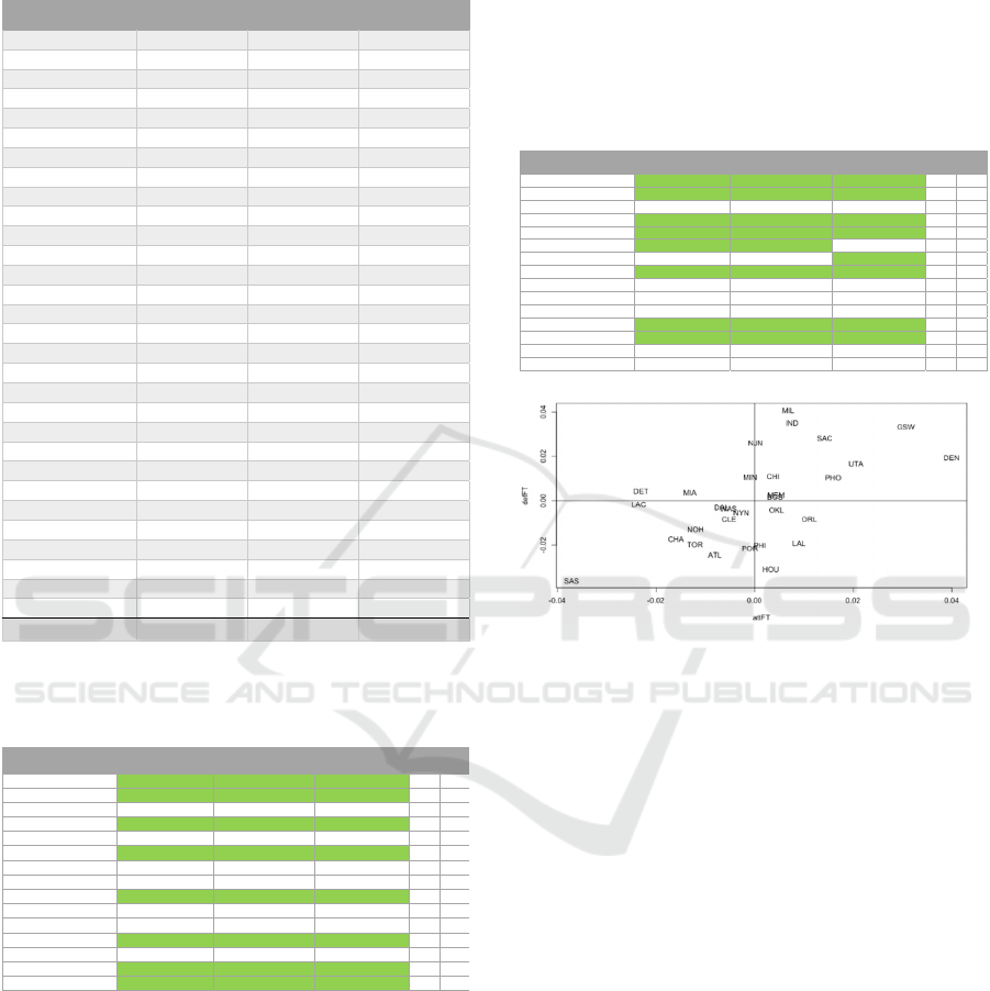
Table 8: Predicted total wins for each team by the Poisson
and negative binomial distributions compared with the real
observations.
Table 9: Predicted final position for each team in the
Western Conference by the Poisson and negative binomial
distributions compared with the real observations.
5.5 Cross-Plots for Team Abilities
Cross-plots on each team’s attack and defence
parameters shall now be shown for for Free Throws
(FT), 2-Point Shots (2PT) and 3-Point Shots (3PT),
respectively. The optimal scenario is for a team to
have a large positive value for their attack strength
and a large negative value for their defense strength
for each specific scoring method. Thus, the bottom
right quadrant of Figure 4 represents the best
combination of attack and defense, whereas the top
left quadrant represents the worst combination.
Cross-plots can be obtained for both the Poisson and
negative binomial models, however only the cross-
plots for the markedly superior model – the negative
binomial model – shall be presented.
Table 10: Predicted final position for each team in the
Eastern Conference by the Poisson and negative binomial
distributions compared with the real observations.
Figure 4: Cross-plot of the estimated means of the posterior
distribution for the attack strength against the estimated
means of the posterior distribution for the defense strength
for each team with respect to Free Throws (FT) from the
negative binomial baseline model.
For Free Throws (FT), the cross-plot in Figure 4
shows that the majority of teams have an attack
parameter value close to the mean except for a few
teams with the Golden State Warriors, Denver
Nuggets and Utah Jazz having the largest values and
the San Antonio Spurs having the smallest value.
Defensively, the teams are a bit more spread out
where the San Antonio Spurs compensate for their
offensive ability by having the smallest value for
defense (i.e. best defensive value) while the
Milwaukee Bucks had the largest value for defense
meaning they conceded the most number of free
throws from all the teams.
For the 2-Point Shots (2PT), Figure 5 shows us
that the best performing team with regards to scoring
2 point shots were the Phoenix Suns while the
Orlando Magic were the team on the opposite end of
the spectrum when it came to scoring 2-Point shots.
With respect to conceding (defense) 2-Point shots, the
New Orleans Hornets had the smallest value with the
Team Name Observed Wins
Predicted Wins
(Negative Binomial)
Predicted Wins
(Poisson)
Atlanta Hawks 47 49 47
Boston Celtics 62 61 75
Charlotte Bobcats 35 37 36
Chicago Bulls 41 41 40
Cleveland Cavaliers 66 64 77
Dallas Mavericks 50 50 50
Denver Nuggets 54 51 57
Detroit Pistons 39 38 34
Golden State Warriors 29 32 24
Houston Rockets 53 52 59
Indiana Pacers 36 35 37
Los Angeles Clippers 19 22 3
Los Angeles Lakers 65 66 74
Memphis Grizzlies 24 25 13
Miami Heat 43 42 43
Milwaukee Bucks 34 35 32
Minnesota Timberwolves 24 22 20
New Jersey Nets 34 34 32
New Orleans Hornets 49 47 48
New York Knicks 32 35 32
Oklahoma City Thunder 23 22 12
Orlando Magic 59 58 73
Philadelphia 76ers 41 43 38
Phoenix Suns 46 46 46
Portland Trail Blazers 54 53 68
Sacramento Kings 17 17 7
San Antonio Spurs 54 53 58
Toronto Raptors 33 32 35
Utah Jazz 48 50 51
Washington Wizards 19 18 9
MAE (Mean Absolute
Prediction Error)
2.67 5.4
Team Name
Observed Final
Position
Predicted Final Position
(Negative Binomial)
Predicted Final
Position (Poisson)
N.B.
+/-
Pois.
+/-
Dallas Mavericks 6
th
6
th
7
th
0 1
Denver Nuggets 2
nd
5
th
5
th
3 3
Golden State Warriors 10
th
10
th
10
th
0 0
Houston Rockets 5
th
4
th
3
rd
1 2
Los Angeles Clippers 14
th
12
th
15
th
2 1
Los Angeles Lakers 1
st
1
st
1
st
0 0
Memphis Grizzlies 11
th
11
th
12
th
0 1
Minnesota Timberwolves 12
th
13
th
11
th
1 1
New Orleans Hornets 7
th
8
th
8
th
1 1
Oklahoma City Thunder 13
th
14
th
13
th
2 0
Phoenix Suns 9
th
9
th
9
th
0 0
Portland Trail Blazers 3
rd
2
nd
2
nd
1 1
Sacramento Kings 15
th
15
th
14
th
0 1
San Antonio Spurs 4
th
3
rd
4
th
1 0
Utah Jazz 8
th
7
th
6
th
1 2
Team Name
Observed Final
Position
Predicted Final Position
(Negative Binomial)
Predicted Final
Position (Poisson)
N.B.
+/-
Pois.
+/-
Atlanta Hawks 4
th
4
th
4
th
0 0
Boston Celtics 2
nd
2
nd
2
nd
0 0
Charlotte Bobcats 10
th
9
th
9
th
1 1
Chicago Bulls 6
th
7
th
6
th
1 0
Cleveland Cavaliers 1
st
1
st
1
st
0 0
Detroit Pistons 8
th
8
th
11
th
0 3
Indiana Pacers 9
th
10
th
8
th
1 1
Miami Heat 5
th
6
th
5
th
1 0
Milwaukee Bucks 11
th
11
th
12
th
0 1
New Jersey Nets 12
th
13
th
14
th
1 2
New York Knicks 13
th
12
th
13
th
1 0
Orlando Magic 3
rd
3
rd
3
rd
0 0
Philadelphia 76ers 7
th
5
th
7
th
2 0
Toronto Raptors 13
th
14
th
10
th
1 3
Washington Wizards 15
t
h
15
t
h
15
t
h
0 0
icSPORTS 2023 - 11th International Conference on Sport Sciences Research and Technology Support
108

Philadelphia 76ers following very closely behind
them. On the other end, the worst defensive
performances came from the Golden State Warriors
and the New York Knicks as they had the largest
values for the 2-Point shot defense parameters.
Figure 5: Cross-plot of the estimated means of the posterior
distribution for the attack strength against the estimated
means of the posterior distribution for the defense strength
for each team with respect to 2-Point Shots (2PT) from the
negative binomial baseline model.
Figure 6: Cross-plot of the estimated means of the posterior
distribution for the attack strength against the estimated
means of the posterior distribution for the defense strength
for each team with respect to 3-Point Shots (3PT) from the
negative binomial baseline model.
Lastly, with respect to 3-Point Shots (3PT), the cross-
plot in Figure 6 shows the New York Knicks and
Orlando Magic having the best attacking ability while
the Oklahoma City Thunder and the Philadelphia
76ers performed the worst when it came to scoring 3-
Point shots. Defensively, the best performing team
was the Detroit Pistons followed by the Orlando
Magic while the Washington Wizards and the
Phoenix Suns had the worst performances with
regards to conceding 3-Point shots.
Table 11: Excerpt of posterior distribution summary
statistics from the winning probability model.
Table 12: Predicted total wins for each team by the
Bernoulli distribution compared with the real observations.
It is interesting to note how the Orlando Magic made
up for their poor 2-Point Shots (2PT) attack strength
by having the second best 3-Point Shots (3PT) attack
strength and also having a Free Throw (FT) attack
strength larger than the mean value. This, together
with all their defensive attributes being better than the
mean value made them one of the best teams that
year. Similar patterns can be noticed for the Los
Angeles Lakers and the Boston Celtics.
5.6 Winning Probability Model Results
and Comparisons with Scoring
Intensity Models
Excerpts of summary statistics for samples from the
posterior distribution of different parameters can be
seen in Table 11. The naïve and time series standard
errors of the parameters were significantly smaller
than they were for the previous setup. Full outputs can
be found in the GitHub repository. The winning
probability model correctly predicts 886 (or 72.03%)
of the total (1230) matches. This is much less than the
predictive accuracy of the negative binomial model,
which correctly predicts 1189 (or 96.67%) of the total
matches, and also less than that of the Poisson model
that predicts 998 (81.3%) of the model. A plot
Parameter Mean Std. Dev. Naive Error TS Error 2.5% Median 97.5%
𝒔𝒕𝒓
𝑨
𝒕𝒍𝒂𝒏𝒕𝒂
0.3308 0.2310 0.0013 0.0017 -0.1221 0.3297 0.7793
𝒔𝒕𝒓
𝑩𝒐𝒔𝒕𝒐𝒏
1.1914 0.2548 0.0015 0.0020 0.7050 1.1874 1.7062
… … … … … … … …
𝒔𝒕𝒓
𝑼𝒕𝒂𝒉
0.3498 0.2308 0.0013 0.0017 -0.0973 0.3472 0.8021
𝒔𝒕𝒓
𝑾𝒂𝒔𝒉𝒊𝒏𝒈𝒕𝒐𝒏
-1.2213 0.2556 0.0015 0.0019 -1.7354 -1.2187 -0.7332
𝜼
0.5639 0.0679 0.0003 0.0005 0.4302 0.5636 0.6966
Team Name Observed Wins Predicted Wins
Atlanta Hawks 47 52
Boston Celtics 62 73
Charlotte Bobcats 35 32
Chicago Bulls 41 39
Cleveland Cavaliers 66 77
Dallas Mavericks 50 56
Denver Nuggets 54 60
Detroit Pistons 39 37
Golden State Warriors 29 21
Houston Rockets 53 59
Indiana Pacers 36 34
Los Angeles Clippers 19 8
Los Angeles Lakers 65 79
Memphis Grizzlies 24 13
Miami Heat 43 41
Milwaukee Bucks 34 29
Minnesota Timberwolves 24 13
New Jersey Nets 34 30
New Orleans Hornets 49 55
New York Knicks 32 27
Oklahoma City Thunder 23 11
Orlando Magic 59 72
Philadelphia 76ers 41 38
Phoenix Suns 46 54
Portland Trail Blazers 54 60
Sacramento Kings 17 9
San Antonio Spurs 54 60
Toronto Raptors 33 30
Utah Jazz 48 55
Washington Wizards 19 6
MAE (Mean Absolute
Prediction Error)
6.93
Bayesian Hierarchical Modelling of Basketball Team Performance: An NBA Regular Season Case Study
109

showing the actual cumulative wins for each team
against those predicted by the winning probability
model can also be found on GitHub
5
.
Table 13: Predicted final position for each team in the
Western Conference by the winning probability model
compared with the real observations.
Table 14: Predicted final position for each team in the
Eastern Conference by the winning probability model
compared with the real observations.
It can be seen that the mean absolute prediction error
for the winning probability model in Table 12 is
considerably inferior to that of the negative binomial
model in Table 11, and also inferior to that of the
Poisson model.
However, it can also be seen in Tables 13 and 14,
that the winning probability model has been just as
effective as the negative binomial model in correctly
predicting all teams which pass through to the
playoffs from both conferences. Furthermore, it has
also proven to be better at predicting the standings
than the negative binomial model. For the Western
conference, the model using the Bernoulli distributed
model showed 2 position changes, while for the
Eastern conference, the Bernoulli distributed model
showed 5.
Finally, for the 2008/2009 NBA season, we also
have the mean of the strength parameters for the
5
bayesianhierarchicalbasketball/CumulativeWP.pdf at main
davidsuda80/bayesianhierarchicalbasketball(github.com)
winning probability model, sorted by the mean
strength, displayed in Figure 7. This plot puts
Cleveland Cavaliers and Los Angeles Lakers at the
very top in terms of strength, while Sacramento Kings
and Los Angeles Clippers are the weakest two (in that
order).
Figure 7: Means plot of the estimated means of the posterior
distribution for the team strength parameter by team (in
descending order) according to the winning probability
model.
6 CONCLUSIONS
In this paper we have analysed the performance of
two Bayesian hierarchical models intended to model
scoring intensity in basketball, based on the Poisson
and negative binomial distributions, and one
Bayesian hierarchical model intended to model the
winning probability in basketball, based on the
Bernoulli distribution. The data under study was
taken to be the NBA 2008/2009 regular season.
It was concluded, from the RMSEs of the different
models and the MAE of the overall prediction on the
number of wins for each team, that making the
negative binomial assumption on the distribution of
the scoring intensities of the different scoring types in
basketball provides a superior performance than
making the Poisson assumption. The negative
binomial model was also better in determining which
teams qualify to the playoffs with 100% accuracy,
while the Poisson model got one team wrong.
Furthermore, the model based on the negative
binomial distribution was also used to determine the
attack and defence strengths of the different teams for
the different scoring types displayed by cross-plots.
The winning probability model, on the other hand,
was inferior to the Poisson type model and, even more
so, the negative binomial type models in predicting
the number of wins for each team. The winning
Team Name Observed Final Position Predicted Final Position
Change
+/-
Dallas Mavericks 6
th
6
th
0
Denver Nuggets 2
nd
2
nd
0
Golden State Warriors 10
th
10
th
0
Houston Rockets 5
th
5
th
0
Los Angeles Clippers 14
th
15
th
1
Los Angeles Lakers 1
st
1
st
0
Memphis Grizzlies 11
th
11
th
0
Minnesota Timberwolves 12
th
12
th
0
New Orleans Hornets 7
th
7
th
0
Oklahoma City Thunder 13
th
13
th
0
Phoenix Suns 9
th
9
th
0
Portland Trail Blazers 3
rd
3
rd
0
Sacramento Kings 15
th
14
th
1
San Antonio Spurs 4
th
4
th
0
Utah Jazz 8
th
8
th
0
Team Name Observed Final Position Predicted Final Position
Change
+/-
Atlanta Hawks 4
th
4
th
0
Boston Celtics 2
nd
2
nd
0
Charlotte Bobcats 10
th
10
th
0
Chicago Bulls 6
th
6
th
0
Cleveland Cavaliers 1
st
1
st
0
Detroit Pistons 8
th
8
th
0
Indiana Pacers 9
th
9
th
0
Miami Heat 5
th
5
th
0
Milwaukee Bucks 11
th
13
th
2
New Jersey Nets 12
th
11
th
1
New York Knicks 13
th
14
th
1
Orlando Magic 3
rd
3
rd
0
Philadelphia 76ers 7
th
7
th
0
Toronto Raptors 13
th
12
th
1
Washington Wizards 15
th
15
th
0
icSPORTS 2023 - 11th International Conference on Sport Sciences Research and Technology Support
110

probability model, however, was just as good as the
negative binomial model for predicting the teams
which qualify to the playoffs, and was even better at
predicting the exact positionings on the scoreboard. A
means plot of the overall strengths of the different
teams could also be obtained for the different teams.
It can therefore be concluded that the negative
binomial model is the superior model when it comes
to predicting specific game outcomes, while the
winning probability model is the superior model
when it comes to predicting final standings as it
proves to be more effective at determining the overall
strengths of each team.
REFERENCES
Baio, G., Blangiardo, M. (2010). Bayesian hierarchical
model for the prediction of football results. In Journal
of Applied Statistics 32(7):253-264. Taylor & Francis.
Boulier, B.L., Stekler, H.O. (1999). Are sports seedings
good predictors? In International Journal of
Forecasting 15:83-91. Science Direct.
Carlin, B.P. (1996). Improved NCAA basketball
tournament modelling via point spread and team
strength information. In The American Statistician,
50(1): 39-43. Taylor & Francis.
Catellan, B.L., Varin, C., Firth, D. (2013). Dynamic
Bradley-Terry modelling of sports tournaments. In
Journal of the Royal Statistical Society Series C –
Applied Statistics, 62:135-150. Wiley.
Caudill, S.B. (2003). Predicting discrete outcomes with the
maximum score estimator: the case of the NCAA men’s
basketball tournament. In International Journal of
Forecasting, 19(2):313-317. Science Direct.
Cervone, D., Bornn, L., Goldsberry, K. (2014). Pointwise:
predicting points and valuing decisions in real time with
NBA optical tracking data. In 8
th
Annual MIT Sloan
Sports Analytics Conference.
Gabrio, A. (2020). Bayesian hierarchical model for the
prediction of volleyball results. In Journal of Applied
Statistics 48(2):301-321. Taylor & Francis.
Gelman, A., Carlin, J., Stern, H.S. (2013). Bayesian Data
Analysis, Chapman and Hall. CRC Press, 3
rd
edition.
Ingram, M. (2019). A point-based Bayesian hierarchical
model to predict the outcome of tennis matches. In
Journal of Quantitative Analysis in Sports 15:313-325.
De Gruyter.
Karlis, D., Ntzoufras, I. (2000). On modelling soccer data.
In Student 3, 229-244.
Karlis, D., Ntzoufras, I. (2003). Analysis of sports data by
using bivariate Poisson models. In Journal of the Royal
Statistical Society Series D – The Statistician, 52:381-
393. Wiley.
Tsionas, E. (2001). Bayesian multivariate Poisson
regression. In Communication in Statistics – Theory
and Methodology, 30(2):243-255. Taylor & Francis.
Bayesian Hierarchical Modelling of Basketball Team Performance: An NBA Regular Season Case Study
111
