Closeness Centrality Detection in Homogeneous Multilayer Networks

Hamza Reza Pavel, Anamitra Roy, Abhishek Santra and Sharma Chakravarthy

Computer Science and Engineering Department and IT Lab, UT Arlington, U.S.A.

Keywords:

Homogeneous Multilayer Networks, Closeness Centrality, Decoupling Approach, Accuracy & Precision.

Abstract:

Centrality measures for simple graphs are well-deﬁned and several main-memory algorithms exist for each.

Simple graphs have been shown to be not adequate for modeling complex data sets with multiple types of

entities and relationships. Although multilayer networks (or MLNs) have been shown to be better suited, there

are very few algorithms for centrality measure computation directly on MLNs. Typically, they are converted

(aggregated or projected) to simple graphs using Boolean AND or OR operators to compute various centrality

measures, which is not only inefﬁcient but incurs a loss of structure and semantics.

In this paper, algorithms have been proposed that compute closeness centrality on an MLN directly using a

novel decoupling-based approach. Individual results of layers (or simple graphs) of an MLN are used and a

composition function is developed to compute the closeness centrality nodes for the MLN. The challenge is

to do this efﬁciently while preserving the accuracy of results with respect to the ground truth. However, since

these algorithms use only layer information and do not have complete information of the MLN, computing a

global measure such as closeness centrality is a challenge. Hence, these algorithms rely on heuristics derived

from intuition. The advantage is that this approach lends itself to parallelism and is more efﬁcient than the

traditional approach. Two heuristics, termed CC1 and CC2, have been presented for composition and their

accuracy and efﬁciency have been empirically validated on a large number of synthetic and real-world-like

graphs with diverse characteristics. CC1 is prone to generate false negatives whereas CC2 reduces them, is

more efﬁcient, and improves accuracy.

1 INTRODUCTION

Closeness centrality measure, a global graph charac-

teristic, deﬁnes the importance of a node in a graph

with respect to its distance from all other nodes. Dif-

ferent centrality measures have been deﬁned, both lo-

cal and global, such as degree (Br

odka et al., 2011),

closeness (Cohen et al., 2014), eigenvector (Sol

et al., 2013), multiple stress (Shi and Zhang, 2011),

betweenness (Brandes, 2001), harmonic (Boldi and

Vigna, 2014), and PageRank (Pedroche et al., 2016).

Closeness centrality deﬁnes the importance of a node

based on how close it is to all other nodes in the graph.

Closeness centrality can be used to identify nodes

from which communication with all other nodes in

the network can be accomplished in least number of

hops. Most of the centrality measures are deﬁned

for simple graphs or monographs. Only page rank

centrality has been extended to multilayer networks

(De Domenico et al., 2015; Halu et al., 2013).

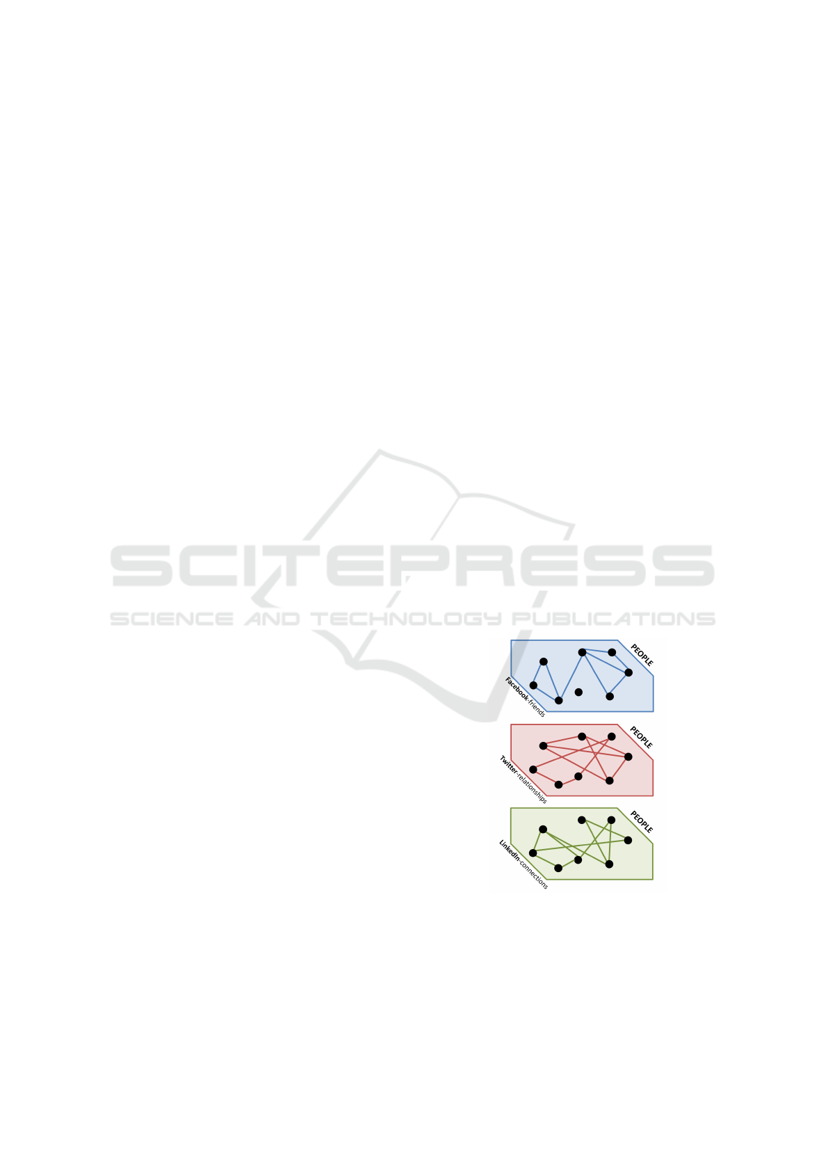
A multilayer network consists of layers, where

each layer is a simple graph consisting of nodes (en-

tities) and edges (relationships) and optionally con-

Figure 1: HoMLN Example.

nected to other layers through inter-layer edges. If

one were to model the three social media networks

Facebook, LinkedIn, and Twitter, an MLN is a better

model as there are multiple edges (connections) be-

tween any two nodes (see Fig. 1.) This type of MLN is

Pavel, H., Roy, A., Santra, A. and Chakravarthy, S.

Closeness Centrality Detection in Homogeneous Multilayer Networks.

DOI: 10.5220/0012159500003598

In Proceedings of the 15th International Joint Conference on Knowledge Discovery, Knowledge Engineering and Knowledge Management (IC3K 2023) - Volume 1: KDIR, pages 17-29

ISBN: 978-989-758-671-2; ISSN: 2184-3228

categorized as homogeneous (or HoMLNs) as the set

of entities in each layer has a common subset, but re-

lationships in each layer are different. It is also possi-

ble to have MLNs where each layer has different types

of entities and relationships within and across layers.

Modeling the DBLP data set (dbl, 1993) with authors,

papers, and conferences needs this type of heteroge-

neous MLNs (or HeMLNs) (Kivel

a et al., 2014).

This paper presents two heuristic-based algo-

rithms to compute closeness centrality nodes (or CC

nodes) on HoMLNs with high accuracy and efﬁ-

ciency. The challenge is in computing a global mea-

sure using partitioned graphs (layers in this case) and

composing them with minimal additional information

to compute a global measure for the combined lay-

ers. Boolean AND composition of layers is used for

ground truth in this paper (OR is another alternative).

These MLN algorithms use the decoupling-based ap-

proach proposed in (Santra et al., 2017a; Santra et al.,

2017b). Based on this approach, closeness centrality

is computed on each layer once and minimal addi-

tional information is kept from each layer to compose.

With this, one can efﬁciently estimate the CC nodes

of the MLN. This approach has been shown to be

application-independent, efﬁcient, lends itself to par-

allel processing (of layers), and is ﬂexible to compute

centrality measure on any arbitrary subset of layers.

Problem Statement: Given a homogeneous MLN

(HoMLN) with l number of layers – G

(V, E

), G

(V, E

), ..., G

(V, E

), where V and E

are the vertex

and edge set in the i

layer – the goal is to identify

the closeness centrality nodes of the Boolean AND-

aggregated layer consisting of any r layers using the

partial results obtained from each of the layers during

the analysis step where r ≤ l. In the decoupling-based

approach, the analysis function is deﬁned as the Ψ

step, and the closeness centrality nodes are estimated

in the composition step or the Θ step using the partial

results obtained during the Ψ step.

1.1 Contributions and Paper Outline

Contributions of this paper are:

• Algorithms for computing closeness centrality

nodes of MLNs

• Two heuristics to improve accuracy and efﬁciency

of computed results

• Use of decoupling-based approach to preserve

structure and semantics of MLNs

• Extensive experimental analysis on large number

of synthetic and real-world-like graphs with di-

verse characteristics.

• Accuracy and Efﬁciency comparisons with

ground truth and naive approach

The rest of the paper is organized as follows: Sec-

tion 2 discusses related work. Section 3 introduces

the decoupling approach for MLN analysis. Sec-

tion 3.1 provides the challenges of decoupling-based

approach for a global metric. Section 4 discusses

the challenges in computing the closeness centrality

nodes in MLNs. Section 5 describes the proposed

heuristics for computing closeness centrality of an

MLN. Section 6 describes the experimental setup and

the data sets. Section 6.1 discusses result analysis fol-

lowed by conclusions in Section 7.

2 RELATED WORK

Due to the rise in popularity and availability of com-

plex and large real-world-like data sets, there is a crit-

ical need for modeling them as graphs and analyz-

ing them in different ways. The centrality measure

of MLN provides insight into different aspects of the

network. Though there have been a plethora of stud-

ies in centrality detection for simple graphs, not many

studies have been done on detecting central entities in

multilayer networks. Existing studies conducted on

detecting central entities in multilayer networks are

use-case speciﬁc and no common framework exists

which can be used to address the issue of detecting

central entities in a multilayer network.

(Cohen et al., 2014) proposes an approach to

ﬁnd top k closeness centrality nodes in large graphs.

This approximation-based approach has higher efﬁ-

ciency under certain circumstances. Even though the

algorithm works on large graphs, unfortunately, it

does not work in the case of multi-layer networks.

In (De Domenico et al., 2015; Sol

e-Ribalta et al.,

2016), authors capitalize on the tensor formalism, re-

cently proposed to characterize and investigate com-

plex topologies, to show how closeness centrality and

a few other popular centrality measures can be ex-

tended to multiplexes. In (Cohen et al., 2014), au-

thors propose a sampling-based approach to estimate

the closeness centrality nodes in undirected and di-

rected graphs with acceptable accuracy. The proposed

approach takes linear time and space but it is a main

memory-based algorithm. The authors of (Sariy

uce

et al., 2013) propose an incremental algorithm that

can dynamically update the closeness centrality nodes

of a graph in case of edge insertion and deletion. The

algorithm has a lower memory footprint compared

to traditional closeness centrality algorithms and pro-

vides massive speedup when tested on real-world-like

graph data sets. In (Du et al., 2015), the authors

KDIR 2023 - 15th International Conference on Knowledge Discovery and Information Retrieval

propose closeness centrality algorithms where they

use effective distance instead of the conventional geo-

graphic distance and binary distance obtained by Di-

jkstra’s shortest path algorithm. This approach works

on directed, undirected, weighted, and unweighted

graphs. In (Putman et al., 2019), authors com-

pute the exact closeness centrality values of all nodes

in dynamically evolving directed and weighted net-

works. This approach is parallelizable and achieves a

speedup of up to 33 times.

Most of the methods to calculate closeness cen-

trality are main memory-based and not suitable

for large graphs. In (Santra et al., 2017b), the

authors propose a decoupling-based approach where

each layer can be analyzed independently and in par-

allel and calculate graph properties for a HoMLN us-

ing the information obtained for each layer. The pro-

posed algorithms are based on the network decou-

pling approach which has been shown to be efﬁcient,

ﬂexible, scalable as well as accurate.

3 DECOUPLING APPROACH FOR

MLNs

Most of the algorithms available to analyze simple

graphs for centrality, community, and substructure

detection cannot be used for MLN analysis directly.

There have been some studies that extend existing al-

gorithms for centrality detection (e.g., page rank) to

MLNs (De Domenico et al., 2015), but they try to

work on the MLN as a whole. The network de-

coupling approach (Santra et al., 2017a; Santra et al.,

2017b) used in this paper not only uses extant algo-

rithms for simple graphs, but also uses a partitioning

approach for efﬁciency, ﬂexibility, and new algorithm

development.

Brieﬂy, existing approaches for multilayer net-

work analysis convert or transform MLN into a single

graph. This is done either by aggregating or project-

ing the network layers into a single graph. For homo-

geneous MLNs, edge aggregation is used to aggregate

the network into a single graph. Although aggregation

of an MLN into a single graph allows one to use ex-

tant algorithms (and there are many of them), due to

aggregation, structure and semantics of the MLN is

not preserved resulting in information loss.

The network decoupling approach is shown in

Figure 2. It consists of identifying two functions: one

for analysis (Ψ) and one for composition (Θ). Us-

ing the analysis function, each layer is analyzed in-

dependently (and in parallel). The results (which are

termed partial from the MLN perspective) from each

of the two layers are then combined using a composi-

tion function/algorithm to produce the results for the

two layers of the HoMLN. This binary composition

can be applied to MLNs with more than two layers.

Independent analysis allows one to use existing algo-

rithms on smaller graphs. The decoupling approach,

moreover, adds efﬁciency, ﬂexibility, and scalability.

Figure 2: Overview of the network decoupling approach.

The network decoupling method preserves struc-

ture and semantics which is critical for drill-down and

visualization of results. As each layer is analyzed in-

dependently, the analysis can be done in parallel re-

ducing overall response time. Due to the MLN model,

each layer (or graph) is likely to be smaller, requires

less memory than the entire MLN, and provides clar-

ity. The results of the analysis functions are saved and

used for the composition. Each layer is analyzed only

once. Typically, the composition function is less com-

plex and is quite efﬁcient, as shall be shown. Any of

the existing simple graph centrality algorithms can be

used for the analysis of individual layers. Also, this

approach is application-independent.

When compared to similar single network ap-

proaches, achieving high accuracy with a decoupling

approach is the challenge, especially for global mea-

sures. While analyzing one layer, identifying mini-

mal additional information needed for improving ac-

curacy due to composition is the main challenge. For

many algorithms that have been investigated, there is

a direct relation between the amount of additional in-

formation used and accuracy gained, however, this af-

fects the efﬁciency.

3.1 Beneﬁts and Challenges of

Decoupling-Based Approach

For analyzing MLNs, currently, HoMLNs are con-

verted into a single graph using aggregation ap-

proaches. Given two vertices u and v, the edges be-

tween them are aggregated into a single graph. The

presence of an edge between vertices u and v depends

on the aggregation function used. In Boolean AND

Closeness Centrality Detection in Homogeneous Multilayer Networks

composed layers, if an edge is present between the

same vertex pair u and v in both layers, then it will

be present in the AND composed layer. Similarly, in

Boolean OR composed layers, if an edge is present

between the same vertex pair u and v in at least one

of the layers in HoMLN, then the edge will be present

in the OR composed layer.

Both HoMLNs and HeMLNs are a set of layers

of single graphs. Hence, the MLN model provides

a natural partitioning of a large graph into layers of

an MLN. The layer-wise analysis as the basis of the

decoupling approach has several beneﬁts. First, the

entire network need not be loaded into memory, only

a smaller layer. Second, the analysis of the individ-

ual layers can be parallelized decreasing the total re-

sponse time of the algorithm. Finally, the computa-

tion used in the composition function (Θ) is based on

intuition which is embedded into the heuristic and re-

quires signiﬁcantly less computation than Ψ.

When analyzing an MLN, the accuracy depends

on the information being kept (in addition to the out-

put) during the analysis of individual layers. In terms

of centrality measures, the bare minimum information

that can be kept from each layer is the high central-

ity (greater than average centrality value) nodes along

with their centrality values. Retaining the minimal in-

formation, local centrality measures like degree cen-

trality can be calculated relatively easily with high ac-

curacy (Pavel et al., 2022) (Pavel. et al., 2022).

However, the calculation of a global measure,

such as closeness centrality nodes, requires informa-

tion of the entire MLN. This compounds the difﬁculty

of computation of closeness centrality of an MLN in

the decoupling approach partial information used for

estimation of the result will greatly impact the accu-

racy. Identiﬁcation of useful minimal information and

the intuition behind that are the primary challenges.

4 CLOSENESS CENTRALITY:

CHALLENGES

The closeness centrality value of a node v describes

how far are the other nodes in the network from v or

how fast or efﬁciently a node can spread information

through the network. For example, when an inter-

net service provider considers choosing a new geo-

location for their servers, they might consider a city

that is geographically closer to most cities in the re-

gion. An airline is interested in identifying a city for

their hub that connects to other important cities with

a minimum number of hops or layovers. For both,

computing the closeness centrality of the network is

the answer.

Figure 3: Closeness centrality for a small toy graph.

The closeness centrality score/value of a vertex u

in a network is deﬁned as,

CC(u) =

n − 1

∑

d(u, v))

(1)

where n is the total number of nodes and d(u, v) is

the shortest distance from node u to some other node

v in the network. The higher the closeness central-

ity score of a node, the more closely (distance-wise)

that node is connected to every other node in the net-

work. Nodes with a closeness centrality score higher

than the average are considered closeness central-

ity nodes (or CC nodes). This deﬁnition of close-

ness centrality is only deﬁned for graphs with a single

connected component. The closeness centrality is de-

ﬁned for both directed and undirected graphs. In this

paper, for an algorithm based on the decoupling ap-

proach, the focus is on the problem of ﬁnding high

(same or above average) closeness centrality nodes

of Boolean AND aggregated layers of an MLN for

undirected graphs. Even though closeness centrality

is not well deﬁned for graphs with multiple connected

components, the heuristics work for networks where

each layer could consist of multiple connected com-

ponents or the AND aggregated layer has multiple

connected components. The proposed heuristics con-

sider the normalized closeness centrality values over

the connected component in the layers (Wasserman

et al., 1994).

For closeness centrality discussed in this paper,

the ground truth (GT) is calculated as follows: i)

Two layers of the MLN are aggregated into a single

graph using the Boolean AND operator and ii) Close-

ness centrality nodes of the aggregated graph are cal-

culated using an existing algorithm. The same algo-

rithm is also used on the layers for calculating CC

nodes of each layer.

For ﬁnding the ground truth CC nodes and identi-

fying the CC nodes in the layers, the NetworkX pack-

age (Hagberg et al., 2008) implementation of close-

ness centrality (Freeman, 1978) (Wasserman et al.,

1994) is used. The implementation of the closeness

centrality algorithm in this package uses breadth-ﬁrst

search (BFS) to ﬁnd the distance from each vertex to

every other vertex. For disconnected graphs, if a node

is unreachable, a distance of 0 is assumed and ﬁnally,

the obtained scores are normalized using Wasserman

KDIR 2023 - 15th International Conference on Knowledge Discovery and Information Retrieval

Figure 4: Layer G

, G

, and AND-aggregated layer created by G

and G

, G

xANDy

(which is computed as G

AND G

)

with the respective closeness centrality of each node. The nodes highlighted in green have above average closeness centrality

values in their respective layers.

and Faust approximation which prioritizes the close-

ness centrality score of vertices in larger connected

components (Wasserman et al., 1994). For a graph

with V vertices and E edges, the time complexity of

the algorithm is O(V (V + E)).

In addition to ground truth, the naive approach

is used for comparing the accuracy of proposed

heuristic-based approaches. In the naive approach,

we take the intersection (as AND aggregation is

being used for GT) of the CC nodes generated for

each layer independently using the same algorithm.

The result of the intersection of nodes is considered

as the CC nodes for the MLN. The naive approach

is the simplest form of composition (using the

decoupling approach) and does not use any additional

information other than the CC nodes from each layer.

The hypothesis is that the naive approach is going to

perform poorly when the topology of the two layers

is very different. Observation 1 illustrates that the

naive composition approach is not guaranteed to

give ground truth accuracy, due to the generation

of false positives and false negatives. One situation

where naive accuracy coincides with the ground truth

accuracy is when the two layers are identical. The

naive accuracy will ﬂuctuate with respect to ground

truth without reaching it in general.

Observation 1. A node that has above average close-

ness centrality value in the AND-aggregated layer

created by G

and G

is not guaranteed to have above

average closeness centrality value in one or both of

the layers G

and G

Example: For single connected component graphs,

assume that an arbitrary node, say u, does not have

above average centrality value in layer G

and layer

. This means that node u has longer paths to reach

every other node in the individual networks. That is,

there exist other nodes, say v, which cover the en-

tire individual networks through shorter paths, thus

having high closeness centrality values. There can be

scenarios in which these other nodes (v) do not have

enough short paths that exist in both layer G

and

layer G

, and as a result bring down their closeness

centrality values (and also the average) in the aggre-

gated layer, G

xANDy

. Here, if the node u, has com-

mon paths from the two layers that are shorter than

the common paths for other nodes, then its closeness

centrality value will go above average in the AND ag-

gregated layer.

This scenario is exempliﬁed by node B in Fig-

ure 4, which in spite of not having above average

closeness centrality value in layers G

and G

, has

above average closeness centrality value in the AND-

aggregated layer, G

xANDy

. It can be observed that the

closeness centrality value for other nodes decreased

signiﬁcantly as they did not have enough common

shorter paths, however, node B, maintained enough

common short paths, thus pushing its closeness cen-

trality value above the average in the AND aggregated

layer.

Hence, it illustrates that a node that has above

average closeness centrality value in the AND-

aggregated layer created by G

and G

is not guaran-

teed to have above average closeness centrality value

in one or both of the layers G

and G

Lemma 1. It is sufﬁcient to maintain, for every pair

of nodes, all paths from the layers, G

and G

, in

order to ﬁnd out the shortest path between the same

nodes in the AND-aggregated layer created by G

and

Closeness Centrality Detection in Homogeneous Multilayer Networks

Proof. Suppose, for every pair of nodes, say u and

v, the set of all paths from the layers G

and G

say P

(u, v) and P

(u, v), respectively, is being main-

tained. Then, by set intersection between P

(u, v)

and P

(u, v), one can ﬁnd out the shortest among the

paths that exist between u and v in both the layers, G

and G

, which is basically the shortest path between

them in the ANDed graph (G

xANDy

) as well. The

common path has to be part of the AND-aggregated

graph by deﬁnition. If there are no common paths, the

AND-aggregation is disconnected and the result still

holds. Figure 4 shows an example. For the nodes

A and F, if it is maintained P

(A, F) = {<(A,F)>,

<(A,B), (B,C), (C,F)>} from layer G

and P

(A, F)

= {<(A,C), (C,F)>, <(A,C), (B,C), (C,F)>, <(A,E),

(E,D), (D,F)>} from layer G

, then one can obtain

the path <(A,C), (B,C), (C,F)> as the shortest com-

mon path, which is the correct shortest path between

these nodes in the ANDed layer, G

xANDy

. The short-

est path from G

between A and F cannot appear in

the ANDed graph. This proves the Lemma 1 that it

is sufﬁcient to maintain all paths between every pair

of nodes to ﬁnd out the shortest paths in the ANDed

layer.

Based on Lemma 1, in the composition step, for

every pair of nodes, the path sets from two layers

need to be intersected to ﬁnd out the shortest com-

mon path. In doing so the closeness centrality value

for each node in the ANDed graph can be calculated.

Clearly, if G

(V, E

) and G

(V, E

) are two layers then

the number of paths between any two nodes will be

(V − 2)!, in the worst case. Thus, the composition

phase will have a complexity of O((V − 2)!(V − 2)!),

which is exponentially higher than the ground truth

complexity O(V (V + min(E

, E

))) and defeats the

entire purpose of the decoupling approach. Thus, the

challenge is to identify the minimum amount of

information to gain the highest possible accuracy

over the naive approach by reducing the number

of false positives and false negatives, without com-

promising on the efﬁciency.

5 CLOSENESS CENTRALITY

HEURISTICS

Two heuristic-based algorithms have been proposed

for computing CC nodes for Boolean AND aggre-

gated layers using the decoupled approach. The ac-

curacy and performance of the algorithms have been

tested against the ground truth. Extensive experi-

ments have been performed on data sets with varying

graph characteristics to show that the solutions work

for any graph and have much better accuracy than the

naive approach. Also, the efﬁciency of the algorithms

is signiﬁcantly better than ground truth computation.

The solution can be extended to MLNs with any num-

ber of layers, where the analysis phase is applied once

and the composition phase is applied as a function of

pairs of partial layer results, iteratively.

Jaccard coefﬁcient is used as the measure to com-

pare the accuracy of the solutions with the ground

truth. Precision, recall, and F1-score have also been

used as evaluation metrics to compare the accuracy

of the solutions. For performance, the execution time

of the solution is compared against that of the ground

truth. The ground truth execution time is computed

as: time required to aggregate the layers using AND

composition function + time required to identify the

CC nodes on the combined graph. The time required

for the proposed algorithms using the decoupling ap-

proach is: max(layer 1, layer 2 analysis times) + com-

position time. The efﬁciency results do not change

much even if the max is not used.

5.1 Closeness Centrality Heuristic CC1

Intuitively, CC nodes in single graphs have high de-

grees (more paths go through it and likely more short-

est paths) or have neighbors with high degrees (sim-

ilar reasoning.) In the ANDed graph (ground truth

graph), CC nodes that are common among both lay-

ers have a high chance of becoming a CC node. More-

over, if a common CC node has high overlap of neigh-

borhood nodes from both layers with above average

degree and low average sum of shortest path (SP) dis-

tances, there is a high chance of that node becoming

a CC node in the ANDed graph. Using this intuition

and observation, heuristic CC1 has been proposed for

identifying CC nodes for two layers as an MLN.

As discussed earlier, in the decoupling approach

the analysis function Ψ is used to analyze the layers

once and the partial results and additional information

in the composition function Θ are used to obtain inter-

mediate/ﬁnal results. For CC1, after the analysis phase

(Ψ) on each layer (say, G

) for each node (say, u), its

degree (deg

(u)) and sum of shortest path distances

(sumDist

(u)), and the one-hop neighbors (NBD

(u))

are maintained if u is a CC node, that is u ∈ CH

When calculating sumDist

(u), if a node v is unreach-

able (which can happen if the graph/layer has multiple

disconnected components), the distance dist(u, v) = n

where n is the number of vertices in the layer (same in

each layer – HoMLN) is considered. This is because

the maximum possible path length in a graph with n

nodes is (n-1).

In the composition phase (Θ), for each vertex

KDIR 2023 - 15th International Conference on Knowledge Discovery and Information Retrieval

(a) Accuracy.: CC1 vs. Naive. (b) Min Ψ vs. Max Θ Times.

Figure 5: Accuracy and Execution Time Comparison: CC1 vs. Naive.

u in each layer (say, G

), the degree distance ratio

(degDistRatio

(u)) is calculated with respect to the

second layer (say, G

) to estimate the likelihood of a

node to be a CC node in the ANDed graph (ground

truth graph) as per equation 2.

degDistRatio

(u) =

sumDist

(u)

min(deg

(u), deg

(u))

(2)

A smaller value of this ratio (i.e. smaller

sum of distances and/or higher degree) means the

vertex u has a higher chance of becoming a CC

node in the ANDed graph. When calculating the

degDistRatio

(u), the degree is estimated for vertex

u in the ANDed graph, by taking into account the up-

per bound of degree, which is min(deg

(u), deg

(u)).

Instead of using the degree of the nodes in each layer,

using the estimated degree of the ground truth graph

gives a better approximation of the ratio value of

the sum of distance and degree for the ground truth

graph. Due to decrease in the edges in the ground

truth graph, the average sum of distances will increase

(as on average, paths will get longer). As a result, the

average degree distance ratio for the ANDed graph,

xANDy

is estimated using equation 3.

avgDegDistRatio

xANDy

max(avgDegDistRatio

, avgDegDistRatio

)

(3)

For each CC node in each layer, the set of central

one-hop nodes, i.e. nodes having the degDistRatio

less than the avgDegDistRatio

xANDy

, is calculated. Fi-

nally, those common CC nodes from the two layers,

which have a signiﬁcant overlap among the central

one-hop neighbors are identiﬁed as the CC nodes of

the ANDed graph, which is given by the set CH

xANDy

The complexity of the composition algorithm is de-

pendent on the ﬁnal step where the overlaps of CC

nodes and their one-hop neighborhoods is considered.

The algorithm will have the worst case complexity of

O(V

) if both layers are complete graphs consisting

of V vertices. Based on the wide variety of data sets

used in experiments, it is believed that the composi-

tion algorithm will have an average case complexity

of O(V ). We are not showing the CC1 composition

algorithm due to space constraints and decided to in-

clude a better composition algorithm (CC2.)

Figure 6: Intuition behind CC2 with example.

Discussion. Experimental results for CC1 are shown

in Section 6.1. Figure 5 shows the accuracy (Jaccard

coefﬁcient) of CC1 compared against the naive ap-

proach on a subset of the synthetic data set 1 (details

in Table 1). Although there is signiﬁcant improve-

ment in accuracy as compared to naive, it is still be-

low 50%. This is seen as a drawback of the heuristic.

Also, composition time is somewhat high for large

graphs. In addition, keeping one-hop neighbors of

the CC nodes of both layers is a signiﬁcant amount

of additional information. Figure 5b shows the maxi-

mum composition time against the minimum analysis

time of the layers (worst case scenario). Even though

Closeness Centrality Detection in Homogeneous Multilayer Networks

the composition time takes less time than the time it

takes for the analysis of layers (one-time cost), the

goal is to further reduce the composition time and the

additional information necessary for the composition

without making any major sacriﬁce to accuracy.

To overcome the above, Closeness Centrality

Heuristic CC2 has been developed, which keeps less

information than CC1, has faster composition time,

and provides better (or same) accuracy.

5.2 Closeness Centrality Heuristic CC2

For heuristic CC1, the estimated value of

avgDegDistRatio

xANDy

is less than or equal to

the actual average degree-distance ratio of the AND

aggregated layer, so false negatives will be generated.

The composition step of CC1 is also computationally

expensive and requires a lot of additional information.

Furthermore, CC1 cannot identify all CC nodes of the

ground truth graph. Closeness centrality heuristic 2

or CC2 has been designed to address these issues.

The design of CC2 is based on estimating the sum

of shortest path (SP) distances for vertices in the

ground truth graph. If the sum of SP distances of a

vertex in the individual layers is known, the upper and

lower limit of the sum of SP distances for that ver-

tex in the ground truth graph can be estimated. This

idea can be intuitively veriﬁed. Let the sum of SP dis-

tances for vertex u in layer G

) be sumDist

(u)

(sumDist

(u).) Let the set of layer G

) edges be

.) In the ground truth graph, the upper bound

for the sum of SP distances of a vertex u is going to

be ∞, if the vertex is disjoint in any of the layers. If

∩E

= E

, the sum of SP distances for any vertex u

in the ground truth graph is going to be sumDist

(u).

If E

⊆ E

, then the ground truth graph will have the

same edges as layer x, and sum of SP distances for

a vertex u in the ground truth graph will be same as

the sum of SP distances for that vertex in layer G

When E

∩ E

= E

, for any vertex u, sumDist

(u) ≥

sumDist

(u) because layer G

will have less edges

than layer G

and average length of SPs in layer G

will be higher than average length of SPs in layer G

Similarly, when E

∩E

= E

, the sum of SP distances

for any vertex u in the ANDed graph is going to be

sumDist

(u) and sumDist

(u) ≥ sumDist

(u). From

the above discussion, it can be said that the sum of SP

distances of a vertex u in the ANDed graph is between

max(sumDist

(u), sumDist

(u)) and ∞.

Algorithm 1 shows the composition step for the

heuristic CC2. In this composition function, it is

assumed that the estimated sum of SP distances of

vertex u is estSumDist

xANDy

(u). sumDist

(u) and

sumDist

(u) are the sum of SP of node u in layer G

Algorithm 1: Procedure for Heuristic CC2.

INPUT: deg

(u), deg

(u), sumDist

(u) ∀u ;

, CH

OUTPUT: CH

xANDy

: estimated CC nodes in ANDed graph

1: for u do

2: estSumDist

xANDy

(u) ←

max(sumDist

(u), sumDist

(u))

3: end for

4: Calculate CH

xANDy

using estSumDist

xANDy

and layer G

respectively, and CH

xANDy

is the esti-

mated set of CC nodes of the ANDed layer. Figure

6 illustrates how the composition function using CC2

is applied on a HoMLN with two layers. For each

node u, the sum of SP is estimated, which is the max-

imum sum of SP of node among the two layers. In

the example, node A has a sum of SP as 9 and 7 in

layer 1 and layer 2, respectively. The estimated sum

of SP of node A will be 9 in the ANDed layer. Simi-

larly, the sum of SP of other vertices can be estimated.

Once the estimated sum of SP of all the vertices in the

ANDed graph is completed, Equation 1 can be used

to calculate the CC values of the nodes in the ANDed

layer. As the CC value for the ANDed layer is cal-

culated using the estimated sum of SP, one can either

take the CC nodes with above-average closeness cen-

trality scores or take the top-k CC nodes. For an MLN

with V nodes in each layer, the worst-case complexity

of the composition algorithm for CC2 is O(V ).

Discussion. Experimental results for CC2 are shown

in Section 6.1. In general, this heuristic gave better

recall as compared to the naive and CC1 approach by

being able to decrease the number of false negatives

(shown in Table 4). Moreover, in terms of accuracy,

both Jaccard coefﬁcient and F1-score (shown in Ta-

ble 5) are better for CC2 as compared to Naive and

CC1 approach, (except a few special cases details on

which are in section 6.1). Also it has been shown em-

pirically that CC2 is much more computationally efﬁ-

cient than CC1.

6 EXPERIMENTAL ANALYSIS

The implementation has been done in Python us-

ing the NetworkX (Hagberg et al., 2008) package.

The experiments were run on SDSC Expanse (Towns

et al., 2014) with single-node conﬁguration, where

each node has an AMD EPYC 7742 CPU with 128

cores and 256GB of memory running the CentOS

Linux operating system.

For evaluating the proposed approaches, both syn-

thetic and real-world-like data sets were used. Syn-

thetic data sets were generated using PaRMAT (Kho-

KDIR 2023 - 15th International Conference on Knowledge Discovery and Information Retrieval

Table 1: Summary of Synthetic Data Set-1.

Base

Graph

Edge

Dist. %

#Edges

#V, #E L1%,L2% L1 L2 L1 AND L2

50KV,

250KE

1 70,30 224976 124988 50319

2 60,40 149982 199983 50392

3 50,50 174980 174977 50422

50KV,

500KE

4 70,30 399962 199986 51374

5 60,40 249978 349954 51458

6 50,50 299971 299960 51541

50KV,

1ME

7 70,30 349955 749892 55158

8 60,40 649918 449935 55647

9 50,50 549933 549922 55896

100KV,

500KE

10 70,30 249989 449970 100412

11 60,40 299986 399978 100494

12 50,50 349983 349981 100493

100KV,

1ME

13 70,30 799937 399978 101695

14 60,40 699948 499969 101822

15 50,50 599958 599964 101998

100KV,

2ME

16 70,30 699949 1499899 106389

17 60,40 1299914 899926 107141

18 50,50 1099924 1099923 107785

150KV,

750KE

19 70,30 674971 374979 150398

20 60,40 449982 599970 150447

21 50,50 524978 524975 150475

150KV,

1.5ME

22 70,30 1199942 599978 151684

23 60,40 749968 1049954 151883

24 50,50 899950 899956 152005

150KV,

3ME

25 70,30 1049951 2249888 156501

26 60,40 1349920 1949906 157295

27 50,50 1649922 1649909 157602

rasani et al., 2015), a parallel version of the popu-

lar graph generator RMAT (Chakrabarti et al., 2004)

which uses the Recursive-Matrix-based graph gener-

ation technique.

For diverse experimentation, for each base graph,

3 sets of synthetic data sets have been generated using

PaRMAT. The generated synthetic data set consists of

27 HoMLNs with 2 layers with varying edge distri-

bution for the layers. The base graphs start with 50K

vertices with 250K edges and go up to 150K vertices

and 3 million edges

. In the ﬁrst synthetic data set,

one layer (L1) follows power-law degree distribution

and the other one (L2) follows normal degree distri-

Graph sizes larger than this could not be run on a single

node due to the number of hours allowed and other limita-

tions of the XSEDE environment.

bution. In the second synthetic data set, both HoMLN

layers have power-law degree distribution. In the ﬁ-

nal synthetic data set, both layers have normal degree

distribution. For each of these, 3 edge distributions

percentages (70, 30; 60, 40; and 50, 50) are used for a

total of 81 HoMLNs of varying edge distributions,

number of nodes and edges for experimentation.

Table 1 shows the details of the different 2-layer

MLNs from the ﬁrst synthetic data set (L1: power-

law, L2: normal) used in the experiments. The other

two synthetic data sets have similar node and edge

distributions.

For the real-world-like data set, the network lay-

ers are generated from real-world like monographs

using a random number generator. The real-world-

like graphs are generated using RMAT with parame-

ters to mimic real world graph data sets as discussed

in (Chakrabarti, 2005). As a result, the graphs have

multiple connected components and also their ground

truth graph.

6.1 Result Analysis and Discussion

In this section, the results of the experiments have

been presented. The two proposed heuristics have

been tested on synthetic and real-world-like data sets

with diverse characteristics. As a measure of accu-

racy, the Jaccard coefﬁcient has been used. The preci-

sion, recall, and F1 scores for the proposed heuristics

have also been compared. As a performance measure,

the time taken by the decoupling approach has been

compared with the time taken to compute the ground

truth (as deﬁned earlier in Section 4.) In addition, the

signiﬁcance of the decoupling approach has also been

highlighted by comparing the maximum composition

time of the proposed algorithms with the minimum

analysis time of the layers. The accuracy of the al-

gorithms is compared against the naive approach that

serves as the baseline for comparison.

Table 2: Accuracy Improvement of CC1 and CC2 over Naive.

Data Set

Mean Accuracy

CC1 CC2 CC1 vs.

Naive

CC2 vs.

Naive

Synthetic-1 43.56% 46.77% +52.57% +63.83%

Synthetic-2 55.95% 55.20% +9.77% +8.30%

Synthetic-3 48.87% 50.90% +47.55% +53.65%

Real-world-like 88.71% 88.2% +7.36% +5.7%

Accuracy. Figure 7 illustrates the accuracy of both

the heuristics and the naive approach against the

ground truth for the synthetic data set-1. As one can

see, the accuracy of the heuristics is better than the

Closeness Centrality Detection in Homogeneous Multilayer Networks

naive approach in all cases. In most cases, CC2 per-

forms better than CC1. The accuracy of CC1 in-

creases with the graph density. A similar trend has

been observed in other synthetic data sets as well,

where the proposed CC1 and CC2 heuristics per-

form better than the naive approach.

Figure 8 shows the accuracy of the algorithms

on real-world-like data sets (distributions mimic real-

world networks(Chakrabarti, 2005)). Across all data

sets, both heuristics have more than 80% accuracy.

The accuracy of the heuristics does not go below the

naive approach even for disconnected graphs. This is

signiﬁcant, as the accuracy of the heuristics based on

intuition is pretty good for real-world-like data sets.

Although some of them show better accuracy for CC1

as compared to CC2, the efﬁciency improvement of

CC2 is an order of magnitude better than CC1 (see

Figure 9).

Table 2 shows the mean accuracy and average per-

centage gain in accuracy over the naive approach for

the synthetic data sets and the real-world-like data set.

For all synthetic data sets, the proposed heuristics sig-

niﬁcantly outperform the naive approach as shown.

The least improvement in accuracy as compared to the

naive approach is only when both layers have power-

law degree distribution. Even for the real-world-like

data set which has a high accuracy for the naive ap-

proach, the heuristics perform better than the naive

approach.

Table 3: Precision of CC1 and CC2 over Naive.

Data Set

Mean Precision

CC1 CC2 CC1 vs. Naive CC2 vs. Naive

Synthetic-1 60.98% 58.08% +1.52% -3.29%

Synthetic-2 74.39% 72.02% -3.10% -6.18%

Synthetic-3 51.99% 52.02% +0.006% +0.0718%

Precision. After comparing the precision values re-

ceived using the proposed heuristics against the ones

from the naive approach for synthetic dataset-1, it is

observed that CC1 has overall better precision com-

pared to the naive approach and CC2. In general, it can

be observed from Table 3, that across different types

of HoMLNs, CC1 and CC2 give high precision values,

ranging from 51% to 74%. However, the improve-

ment over naive is marginal in most of the cases.

For synthetic data sets where one layer has normal

degree distribution and the other layer has power-law

degree distribution, CC2 precision drops slightly. CC2

was developed mainly to increase efﬁciency and pre-

serve accuracy.

Recall. After comparing the recall values received

using the proposed heuristics against the ones from

the naive approach for synthetic data set 1, it is ob-

Table 4: Recall Improvement of CC1 and CC2 over Naive.

Data Set

Mean Recall

CC1 CC2 CC1 vs.

Naive

CC2 vs.

Naive

Synthetic-1 60.38% 71.01% +70.87% 100%

Synthetic-2 72.79% 71.38% +16.71% +14.47%

Synthetic-3 48.87% 50.89% +47.55% +53.65%

served that CC2 has overall better recall compared to

the naive approach and CC1. In general, it can be

observed from Table 4 that across different types of

HoMLNs, both CC1 and CC2 have higher recall

values than the naive approach. Here, the heuris-

tics achieve high recall values in the range from 49%

to 73%. It is observed that the proposed heuristics are

able to decrease the false negatives more as compared

to naive approach, which explains their marked im-

provement in terms of recall. However, the improve-

ment over naive is marginal in most of the cases.

Table 5: F1-Score Improvement of CC1 and CC2 over Naive.

Data Set

Mean F1-Score

CC1 CC2 CC1 vs. Naive CC2 vs. Naive

Synthetic-1 60.58% 63.80% +36.56% +43.80%

Synthetic-2 71.67% 71.09% +6.21% +5.3%

Synthetic-3 50.22% 51.36% +24.71% +27.53%

F1-Score. On comparing the F1-score received us-

ing the proposed heuristics against the ones from the

naive approach for synthetic data set 1, it is observed

that CC2 has an overall better F1-score compared to

the naive approach and CC1. It is established from

Table 5 that across different types of HoMLNs, both

CC1 and CC2 have higher F1-scores than the naive

approach, reaching as high as 72%.

Performance. The ground truth graph obtained from

Boolean AND operation on layers of HoMLN will al-

ways have same or less number of edges than the in-

dividual layers as an edge will appear in the ground

truth graph only if it is connected between the same

nodes in both the layers. The NetworkX (Hagberg

et al., 2008) package used here utilizes BFS to calcu-

late the summation of distances from a node to every

other node while calculating the normalized closeness

centrality of the nodes. As the complexity of BFS de-

pends on the number of vertices and edges in a graph,

the ground truth will always require same or less time

than the analysis time for the largest layer.

Although the sum of the analysis time of the lay-

ers may be more than that of the ground truth, one

needs to only consider the maximum analysis time of

layers as they can be done in parallel. Furthermore,

the composition time is drastically less than the anal-

KDIR 2023 - 15th International Conference on Knowledge Discovery and Information Retrieval

Figure 7: Accuracy Comparison for Synthetic Data Set-1 (Refer Table 1 where Graph Pair ID is G

Figure 8: Accuracy of the heuristics CC1 and CC2 for the real-world-like data sets.

Figure 9: Performance Comparison of CC1 and CC2 on

Largest Synthetic Data Set 1: Min. Ψ Time vs. Max. CC1

Θ Time vs. Max CC2 Θ Time (worst case scenario).

ysis time of any layer. Hence, the minimum analysis

time for layers is compared with the maximum com-

position time to show the worst case scenario. As can

be seen from Figure 9 (plotted on log scale), the max-

imum CC1 composition time is at least 80% faster

and CC2 is an order of magnitude faster than the

minimum analysis time! In addition, the layer analy-

sis is performed once and used for all subset CC node

computation of n layers (which is exponential on n).

Discussion. Both proposed heuristics are better than

the naive approach in terms of accuracy and way more

efﬁcient than ground truth computation. CC2 is better

than CC1 if overall accuracy and efﬁciency are con-

sidered, but CC1 performs better than CC2 for high-

density graphs and has better precision. The availabil-

ity of multiple heuristics and their efﬁcacy on accu-

racy and efﬁciency allows one to choose appropriate

heuristics based on graph/layer characteristics.

Closeness Centrality Detection in Homogeneous Multilayer Networks

7 CONCLUSIONS AND FUTURE

WORK

In this paper, decoupling-based algorithms for com-

puting a global graph metric - closeness centrality -

directly on MLNs have been presented. Two heuris-

tics (CC1 and CC2) were developed to improve accu-

racy over the naive approach. CC2 gives signiﬁcantly

higher accuracy than naive for graphs on a large num-

ber of synthetic graphs and graphs that are real-world-

like with varying characteristics. CC2 is extremely

efﬁcient as well. Future work is to extend the algo-

rithms to more than 2 layers and improve accuracy.

ACKNOWLEDGMENTS

This work was partly supported by NSF Grants CCF-

1955798 and CNS-2120393.

REFERENCES

(1993). Dblp: Digital bibliography & library project. dblp.

org.

Boldi, P. and Vigna, S. (2014). Axioms for centrality. In-

ternet Mathematics, 10(3-4):222–262.

Brandes, U. (2001). A faster algorithm for betweenness

centrality. The Journal of Mathematical Sociology,

25(2):163–177.

odka, P., Skibicki, K., Kazienko, P., and Musiał, K.

(2011). A degree centrality in multi-layered social

network. In 2011 International Conf. CASoN, pages

237–242.

Chakrabarti, D. (2005). Tools for large graph mining.

Carnegie Mellon University.

Chakrabarti, D., Zhan, Y., and Faloutsos, C. (2004). R-mat:

A recursive model for graph mining. In Proceedings

of the 2004 SIAM International Conference on Data

Mining, pages 442–446. SIAM.

Cohen, E., Delling, D., Pajor, T., and Werneck, R. F. (2014).

Computing classic closeness centrality, at scale. In

Proceedings of the second ACM conference on Online

social networks, pages 37–50.

De Domenico, M., Sol

e-Ribalta, A., Omodei, E., G

omez,

S., and Arenas, A. (2015). Ranking in interconnected

multilayer networks reveals versatile nodes. Nature

Communications, 6(1).

Du, Y., Gao, C., Chen, X., Hu, Y., Sadiq, R., and Deng,

Y. (2015). A new closeness centrality measure via

effective distance in complex networks. Chaos:

An Interdisciplinary Journal of Nonlinear Science,

25(3):033112.

Freeman, L. C. (1978). Centrality in social networks con-

ceptual clariﬁcation. Social networks, 1(3):215–239.

Hagberg, A., Swart, P., and S Chult, D. (2008). Explor-

ing network structure, dynamics, and function using

networkx. Technical report, Los Alamos National

Lab.(LANL), Los Alamos, NM (United States).

Halu, A., Mondrag

on, R. J., Panzarasa, P., and Bianconi, G.

(2013). Multiplex pagerank. PLOS ONE, 8(10):1–10.

Khorasani, F., Gupta, R., and Bhuyan, L. N. (2015). Scal-

able simd-efﬁcient graph processing on gpus. In

Proceedings of the 24th International Conference on

Parallel Architectures and Compilation Techniques,

PACT ’15, pages 39–50.

Kivel

a, M., Arenas, A., Barthelemy, M., Gleeson, J. P.,

Moreno, Y., and Porter, M. A. (2014). Multilayer net-

works. Journal of Complex Networks, 2(3):203–271.

Pavel, H., Roy, A., Santra, A., and Chakravarthy, S. (2022).

Degree centrality deﬁnition, and its computation for

homogeneous multilayer networks using heuristics-

based algorithms. In International Joint Conference

on Knowledge Discovery, Knowledge Engineering,

and Knowledge Management, pages 28–52. Springer.

Pavel., H. R., Santra., A., and Chakravarthy., S. (2022).

Degree centrality algorithms for homogeneous mul-

tilayer networks. In Proceedings of the 14th In-

ternational Joint Conference on Knowledge Discov-

ery, Knowledge Engineering and Knowledge Manage-

ment (IC3K 2022) - KDIR, pages 51–62. INSTICC,

SciTePress.

Pedroche, F., Romance, M., and Criado, R. (2016). A biplex

approach to pagerank centrality: From classic to mul-

tiplex networks. Chaos: An Interdisciplinary Journal

of Nonlinear Science, 26(6):065301.

Putman, K. L., Boekhout, H. D., and Takes, F. W. (2019).

Fast incremental computation of harmonic closeness

centrality in directed weighted networks. In 2019

IEEE/ACM International Conference on Advances in

Social Networks Analysis and Mining (ASONAM),

pages 1018–1025.

Santra, A., Bhowmick, S., and Chakravarthy, S. (2017a).

Efﬁcient community re-creation in multilayer net-

works using boolean operations. In International Con-

ference on Computational Science, ICCS 2017, 12-14

June 2017, Zurich, Switzerland, pages 58–67.

Santra, A., Bhowmick, S., and Chakravarthy, S. (2017b).

Hubify: Efﬁcient estimation of central entities across

multiplex layer compositions. In IEEE International

Conference on Data Mining Workshops.

Sariy

uce, A. E., Kaya, K., Saule, E., and C¸ atalyiirek,

U. V.

(2013). Incremental algorithms for closeness central-

ity. In 2013 IEEE International Conference on Big

Data, pages 487–492.

Shi, Z. and Zhang, B. (2011). Fast network centrality anal-

ysis using gpus. BMC Bioinformatics, 12(1).

Sol

a, L., Romance, M., Criado, R., Flores, J., Garc

ıa del

Amo, A., and Boccaletti, S. (2013). Eigenvector

centrality of nodes in multiplex networks. Chaos:

An Interdisciplinary Journal of Nonlinear Science,

23(3):033131.

Sol

e-Ribalta, A., De Domenico, M., G

omez, S., and Are-

nas, A. (2016). Random walk centrality in intercon-

nected multilayer networks. Physica D: Nonlinear

KDIR 2023 - 15th International Conference on Knowledge Discovery and Information Retrieval

Phenomena, 323-324:73–79. Nonlinear Dynamics on

Interconnected Networks.

Towns, J., Cockerill, T., Dahan, M., Foster, I., Gaither, K.,

Grimshaw, A., Hazlewood, V., Lathrop, S., Lifka, D.,

Peterson, G. D., Roskies, R., Scott, J., and Wilkins-

Diehr, N. (2014). Xsede: Accelerating scientiﬁc

discovery. Computing in Science and Engineering,

16(05):62–74.

Wasserman, S., Faust, K., et al. (1994). Social network anal-

ysis: Methods and applications.

Closeness Centrality Detection in Homogeneous Multilayer Networks