
Closing the Sim-to-Real Gap with Physics-Enhanced Neural ODEs
Tobias Kamp
a
, Johannes Ultsch
b
and Jonathan Brembeck
c
German Aerospace Center, Institute of System Dynamics and Control (SR), Germany
Keywords:
Dynamical Systems, Hybrid Modelling, Neural Ordinary Differential Equations, Scientific Machine Learning,
Physics-Enhanced Neural ODEs.
Abstract:
A central task in engineering is the modelling of dynamical systems. In addition to first-principle methods,
data-driven approaches leverage recent developments in machine learning to infer models from observations.
Hybrid models aim to inherit the advantages of both, white- and black-box modelling approaches by combin-
ing the two methods in various ways. In this sense, Neural Ordinary Differential Equations (NODEs) proved
to be a promising approach that deploys state-of-the-art ODE solvers and offers great modelling flexibility. In
this work, an exemplary NODE setup is used to train low-dimensional artificial neural networks with phys-
ically meaningful outputs to enhance a dynamical model. The approach maintains the physical integrity of
the model and offers the possibility to enforce physical laws during the training. Further, this work outlines
how a confidence interval for the learned functions can be inferred based on the deployed training data. The
robustness of the approach against noisy data and model uncertainties is investigated and a way to optimize
model parameters alongside the neural networks is shown. Finally, the training routine is optimized with mini-
batching and sub-sampling, which reduces the training duration in the given example by over 80 %.
1 INTRODUCTION
The modelling of dynamical systems is an impor-
tant and challenging engineering task which forms
the foundation for subsequent controller design, op-
timization, visualization and many more. Models are
usually optimized for specific applications, since ex-
act (white-box) modelling of complex systems soon
becomes infeasible. In order to optimize a model re-
garding its prediction quality or computational com-
plexity, conventional data-driven approaches like pa-
rameter optimization, system identification and the
usage of look-up tables are common practice.
Black-Box Modelling
With the rise of machine learning (ML) algorithms
and toolboxes, manifold data-driven modelling ap-
proaches for dynamical systems emerged. Espe-
cially recurrent neural networks (RNNs) proved to
be well suited to learn time-dependent correlations
(Haber and Ruthotto, 2017), (Chang et al., 2019).
Neural Ordinary Differential Equations (NODEs), as
a
https://orcid.org/0009-0006-5584-2928
b
https://orcid.org/0000-0001-6483-8468
c
https://orcid.org/0000-0002-7671-5251
introduced by Chen (Chen et al., 2018), pose an-
other promising approach. NODEs only approxi-
mate the right-hand side of the differential equations
with neural networks (NNs) and benefit from the us-
age of well-established ODE solvers that enable time-
continuous simulation and the handling of stiff sys-
tems and time events. However, pure black-box ap-
proaches generally suffer from poor extrapolation,
high data demand and instability. Knowledge of the
fundamental dynamics of a system can be used to mit-
igate these disadvantages using a hybrid modelling
approach.
Hybrid Modelling
Hybrid models combine first-principle methods with
machine learning and aim to leverage the advan-
tages of both. One way to use the existing knowl-
edge is to enforce physically meaningful behaviour
of the black-box model during the training. Raissi in-
troduced Physics-informed neural networks (PINNs)
(Raissi et al., 2019) to solve problems that involve
partial differential equations. These networks lever-
age the power of automatic differentiation to incor-
porate knowledge about the derivatives into the loss
function. Another way to use the physical equations is
the explicit combination with black-box components.
Kamp, T., Ultsch, J. and Brembeck, J.
Closing the Sim-to-Real Gap with Physics-Enhanced Neural ODEs.
DOI: 10.5220/0012160100003543
In Proceedings of the 20th International Conference on Informatics in Control, Automation and Robotics (ICINCO 2023) - Volume 2, pages 77-84
ISBN: 978-989-758-670-5; ISSN: 2184-2809
Copyright © 2023 by SCITEPRESS – Science and Technology Publications, Lda. Under CC license (CC BY-NC-ND 4.0)
77

In this case, the white-box part serves e.g. to pre-
process the inputs, initialize hidden states of recur-
rent architectures or to provide an a-priori estimation
that is afterwards corrected by data-driven compo-
nents (cf. residual-physics, (Daw et al., 2022), (Zeng
et al., 2020)). The idea of residual-physics formed the
basis for dedicated hybrid simulators which allow the
incorporation and training of NNs in physics-based
models (Ajay et al., 2018), (Heiden et al., 2020). For
a more complete overview of current developments
in hybrid modelling, we refer the interested reader to
the surveys of Willard (Willard et al., 2020), Rai (Rai
and Sahu, 2020) and Karniadakis (Karniadakis et al.,
2021).
Universal Differential Equations
Universal differential equations (UDEs) (Rackauckas
et al., 2020) expand the basic idea of Neural ODEs
and allow arbitrary designs of the differential equa-
tions. This enables the enrichment of dynamical
models with NNs to expand or replace equations or
computational costly parts. The concept was used
in several works and in different domains, for in-
stance in vehicle dynamics (Bruder and Mikelsons,
2021), (Thummerer et al., 2022), chemistry (Owoyele
and Pal, 2022), climate modelling (Ramadhan et al.,
2022) or fluid dynamics (Thummerer et al., 2021).
Contribution
The generality and physical integrity of a hybrid
model diminishes with increasing influence and com-
plexity of its black-box components, while the de-
mand for training data rises. In the reviewed ap-
plications of NODEs, the physical model is either
combined with data-driven components to form a
higher-order model (Thummerer et al., 2021), (Thum-
merer et al., 2022) or the NNs approximate the right-
hand side of single differential equations (Bruder and
Mikelsons, 2021), (Owoyele and Pal, 2022). While
the obtained models demonstrate the potentials of hy-
brid approaches, y NODEs are prone to instability is-
sues and/or local optima (Turan and Jaschke, 2022)
and the analysis of the physical feasibility and extrap-
olation is not trivial. Inspired by the idea of “fine-
grained data-driven models” (Heiden et al., 2020), we
propose to go one step deeper and insert physically
meaningful neural components into the given differ-
ential equations, forming a Physics-enhanced NODE
(PeNODE). This has the advantage, that the learned
functions can be analysed directly and physical prop-
erties can be enforced during the training. In addi-
tion, we show how a confidence interval can be de-
rived from the training data, which serves to define
the application boundaries of the hybrid model. An-
other benefit of the presented approach is the limited
influence of the data-driven components, which re-
duces stability and convergence issues and minimises
the data-demand.
Outline
This work is structured as follows: In Section 2, we
present the concept of PeNODEs and how the loss-
function can be used to enforce physical laws. In
Section 3, the training routine and the benefits of
mini-batching and sub-sampling are described. Our
demonstrator, a quarter vehicle model, is introduced
in Section 4. The conducted experiments and cor-
responding results are presented in Section 5 before
concluding with Section 6.
2 METHOD
This section presents a method to formulate PeN-
ODEs and how to enforce properties with regularizing
terms. Further, the idea of simultaneous parameter fit-
ting is introduced.
2.1 Terminology
The meaningful combination of physical equations
and NNs is referred to as Physics-enhanced Neu-
ral ODE (PeNODE). The additional usage of reg-
ularizing terms that guide the optimization and en-
force certain properties would be a “Physics-Informed
Physics-enhanced Neural ODE” (cf. PINNs, (Raissi
et al., 2019)). For the sake of simplicity, we however
assume that a Physics-enhanced Neural ODE can also
be Physics-Informed.
2.2 Prerequisites
This work postulates the existence of a dynamical
model, which fairly represents the fundamental dy-
namics of the considered system. The model must be
given in the general form
˙x(t) = f (x,u,t) (1)
y(t) = g(x,u,t) , (2)
with a state-vector x, input-vector u and output-vector
y.
2.3 Deriving a PeNODE
In order to obtain a neural ODE, the right-hand side
of the differential equation (1) is enhanced with one
ICINCO 2023 - 20th International Conference on Informatics in Control, Automation and Robotics
78

or more NNs with parameters Θ:
˙x(t) = f (x,u,t, NN(x,u,t, Θ)) . (3)
The analogy of systems in different domains (Hogan
and Breedveld, 2005) offers the possibility to sketch
a general approach to obtain a PeNODE, i.e. a mean-
ingful combination of the physical equations and
NNs:
In the context of systems analogy, the three ba-
sic components of a dynamical system are compli-
ance, inductance and resistance. Further, a domain-
specific pair of power conjugated variables, i.e. one
flow variable and one potential variable can be de-
fined. Component-specific (differential-) equations
correlate flow and potential (e.g. U = RI for an
electrical resistance) and/or define the transition to
another domain. The differential equations of the
system can be derived by setting the potentials to
be equal and the sum of flows equal to zero for
each connection of the components and substitute the
component-specific equations (Zimmer, 2016).
Based on the described formalism, we propose to
introduce neural components into the systems equa-
tions that obey the same fundamental rules and learn
the correlation of flow and potential. The number
of relevant inputs for these neural components is ex-
pected to be low, since they capture but one aspect
of the complex system they compose. The NNs thus
have a low-dimensional input and an one-dimensional
output. This “fine-grained” approach is advanta-
geous, because the obtained neural components are
easy to analyse regarding their physical feasibility
and extrapolation properties. Furthermore, physically
meaningful behaviour can be encouraged during the
training by punishing unphysical outputs. Finally, the
limited influence of the black-boxes avoids stability
issues and minimises the data demand.
The presented approach is well suited to enhance
models which already capture the fundamental dy-
namics of the real system. In this case, the neural
components can account for secondary effects like
friction, elasticities or non-linear characteristics that
cause the Sim-to-Real Gap, i.e. the residuum between
model predictions and real observations.
2.4 Physics-Informed Training
During the training, the parameters of the neural com-
ponents are adapted to minimise the error (or loss) of
the model-predictions with respect to given training
data. In order to obtain physically reasonable neu-
ral components, regularizing terms that punish un-
physical behaviour can be added to the loss function.
For example, zero-crossing of learned functions is de-
sirable in many cases: Consider a neural resistance
(damper) with trainable parameters Θ which intro-
duces a damper force F
R,NN
(v) that depends on a ve-
locity v. For v = 0, this force must be equal to zero.
Thus, a possible regularizing term is given by
r
zcross
(Θ) = F
R,NN
(0,Θ)
2
. (4)
Since a regularizing term in the loss function cannot
enforce exact zero-crossing, the remaining offset can
be eliminated after the training by subtraction:
˜
F
R,NN
(v) = F
R,NN
(v) − F
R,NN
(0) . (5)
If secondary dependencies, i.e. more inputs are added
to the neural component, the concepts of regularizing
and offset-correction are still applicable. In that case,
the zero-crossing values of arbitrary sample points of
the input space of the secondary inputs can be used for
the regularization. In the given example, if a depen-
dency of the temperature T is added, the regularizer
can be adapted to
r
zcross
(Θ) =
1
N
N
∑
i=0
F
R,NN
(0,T
i
,Θ)
2
, (6)
with N samples from the temperature input-space.
The given example shows how a regularizer for a
single neural component can be formulated. In addi-
tion to such specific terms, general knowledge about
system properties like stability and oscillation capa-
bility can be incorporated using eigen-informed regu-
larizers (Thummerer and Mikelsons, 2023).
2.5 Optimizing Model Parameters
The presented approach relies on low-dimensional
NNs whose influence is limited by design. In order
to add further degrees of freedom to the optimiza-
tion, certain model parameters, e.g. the masses or
inertia, can be optimized alongside the parameters of
the NNs. To optimize model parameters {p
1
, p
2
,...},
we propose to define a vector of parameter-modifiers
P
∆
= [δp
1
, δp
2
,...]
T
that is concatenated with the
vector of the NN-parameters and subjected to the
gradient-based optimization. To ensure stability of
the model and limit the impact of the modifiers, a
smooth saturation with a hyperbolic tangent function
can be used. The modified model parameters ˜p
i
are
then given by
˜p
i
= (1 + δp
i
)p
i
(7)
δp
i
= γtanh(δp
i
) . (8)
The hyper-parameter γ ∈ (0, 1) ensures that the pa-
rameters can only be changed by max . ± γ, e.g.
±20 %.
Closing the Sim-to-Real Gap with Physics-Enhanced Neural ODEs
79

3 TRAINING DETAILS
In this section, the training process for a NODE is
briefly sketched, revealing how mini-batching and
sub-sampling help to reduce the computational com-
plexity and how to use model outputs as physical fea-
tures.
3.1 Basic Training
The basic training routine of a NODE is to repeat-
edly simulate the model for a given time horizon, cal-
culate the loss with respect to all or a subset of the
states and adapt the weights of the NNs in a step
of a gradient-based algorithm, e.g. gradient descent.
The loss function can be any common metric like the
(root) mean squared error over all time-points and
states. The gradient-based optimization requires the
usage of a differentiable ODE-solver, as provided in
Julia (Bezanson et al., 2017) or PyTorch
1
. This con-
sequently assumes that the model is (re)implemented
in the training environment. With FMIFlux.jl
2
, the
model exchange standard FMI
3
can be used to facili-
tate this process and integrate FMUs into Julia appli-
cations.
3.2 Mini-Batching and Sub-Sampling
The computational complexity of the gradient calcu-
lation increases significantly with the length and sam-
ple rate of the deployed training trajectories. Mini-
batching can be used to eliminate this effect and make
the training scalable to arbitrary datasets by using a
number of short sequences from the original dataset
for each update. A further reduction of complex-
ity can be achieved by sub-sampling, i.e. calculat-
ing the loss for a subset of the data points. To intro-
duce randomness and avoid aliasing, the points can be
sampled randomly instead of using equidistant time-
intervals.
3.3 Model Outputs as Physical Features
In many cases, not all states of a system are mea-
surable with reasonable effort. While methods for
state estimation can be used to fill in missing mea-
surements, the NODE can also be trained on a subset
of states or other quantities. In this case, the model
observation function (cf. Equation (2)) is used to
transform the state trajectory into an output trajectory
1
https://github.com/rtqichen/torchdiffeq
2
https://github.com/ThummeTo/FMIFlux.jl
3
https://fmi-standard.org/
which reflects the available measurements. Using the
model outputs for the training is a form of feature ex-
traction and can serve to condense the possibly high-
dimensional state-space to a set of (relevant) quanti-
ties. Note, that if measurement for states are missing,
the usage of mini-batching is impeded, since the ini-
tial state for each sequence must be given to solve the
differential equations correctly.
4 DEMONSTRATOR
In this section we introduce our demonstrator, a quar-
ter vehicle model (QVM). A non-linear version of the
QVM serves to generate training data and the linear
QVM is transformed into a PeNODE that is used in
several training-setups to demonstrate our method.
4.1 The Linear QVM
The QVM is commonly used to represent the vertical
dynamics of road vehicles. It consists of two masses,
one for the wheel (m
w
) and one for one quarter of
the body (m
b
) (cf. Figure 1). The two masses are
connected by a linear spring-damper pair with coeffi-
cients c
s
and d
s
, representing the vehicle suspension
(index s). Another linear spring-damper pair with co-
efficients c
t
and d
t
represents the tire that connects the
vehicle to the ground (index t). The state vector x con-
sists of the road height z
r
, the position and velocity of
the wheel z
w
and v
w
and the position and velocity of
the body z
b
and v
b
. The input u(t) is the differential
road height ˙z
r
and the model output y contains the ac-
celerations of the wheel and the body a
w
and a
b
.
x = [x
1
,...,x
5
]
T
= [z
b
, v
b
, z
w
, v
w
, z
r
]
T
(9)
y = [ ˙x
2
, ˙x
4
]
T
= [a
b
, a
w
]
T
(10)
u = ˙z
r
(11)
The linear differential equations that describe the sys-
tem (12 - 16) can be derived using the Newtonian laws
of motion.
˙x
1
= v
b
(12)
˙x
2
= m
−1
b
(c
s
∆z
s
+ d
s
∆v
s
) (13)
˙x
3
= v
w
(14)
˙x
4
= m
−1
w
(c
t
∆z
t
+ d
t
∆v
t
− c
s
∆z
s
− d
s
∆v
s
) (15)
˙x
5
= u (16)
∆z
s
= z
w
− z
b
, ∆v
s
= v
w
− v
b
∆z
t
= z
r
− z
w
, ∆v
t
= ˙z
r
− v
w
ICINCO 2023 - 20th International Conference on Informatics in Control, Automation and Robotics
80

m
b
m
w
c
s
d
s
c
t
d
t
z
r
z
w
z
b
∆z
s
F
NN,c
F
NN,d
P
∆
∆v
s
Figure 1: Scheme of the hybrid quarter vehicle model with
the incorporated black-box components.
4.2 Data Generation
For the generation of training data, the linear QVM
is extended by two non-linear effects in the suspen-
sion. A translational friction force F
f r
, consisting
of Stribeck-, Coulomb and viscous friction, is added
(cf. Simscape: Translational Friction
4
) and the spring
is modified towards a progressive characteristic by
adding a quadratic term F
pr
. The model equations
(13) and (15) are consequently changed to
˙x
2
= m
−1
b
(c
s
∆z
s
+ d
s
∆v
s
+ F
pr
(∆z
s
) + F
f r
(∆v
s
)) (17)
˙x
4
= m
−1
w
(c
t
∆z
t
+ d
t
∆v
t
− c
s
∆z
s
− d
s
∆v
s
− F
pr
(∆z
s
) − F
f r
(∆v
s
)) . (18)
To obtain the trajectory of states and outputs, the non-
linear model is simulated over time for a given input
u(t). The input is derived from a realistic road profile
(ISO8608, Type D (M
´
u
ˇ
cka, 2017)), imitating a rather
rough road. The generated states and observables are
sampled with 1000 Hz and are artificially disturbed
by Gaussian noise. The training dataset consists of a
single trajectory of 42 s length.
4.3 The Neural QVM
For the demonstration of our method, the basic linear
model is augmented with two NNs to learn the miss-
ing effects from the data. The NNs are interpreted as
neural compliance and -resistance (here: spring and
damper) that induce the forces F
NN,c
and F
NN,d
. They
consequently add to the sum of forces in the given
4
https://www.mathworks.com/help/simscape/ref/
translationalfriction.html, accessed 27.04.2023
Table 1: Architecture of the deployed neural networks.
Layer Dimensions Activation
1 16 × 1 ReLU
2 16 × 16 ReLU
3 1 × 16 Identity
differential equations according to:
˙x
2
= m
−1
b
(c
s
∆z
s
+ d
s
∆v
s
+ F
NN,c
(∆z
s
)
+ F
NN,d
(∆v
s
)) (19)
˙x
4
= m
−1
w
(c
t
∆z
t
+ d
t
∆v
t
− c
s
∆z
s
− d
s
∆v
s
− F
NN,c
(∆z
s
) − F
NN,d
(∆v
s
)) . (20)
The architecture of the neural networks is summa-
rized in Table 1. In our approach, the neural compo-
nents capture single effects within a complex system.
In most cases, the learned functions will be simple
and small NNs with few nodes suffice. In the given
setup, the two NNs only have 321 parameters each.
In a realistic setup, the accelerations a
b
and a
w
are
comparably easy to measure. Therefore, the model
output y is used for the optimization. The loss func-
tion is a normalized root mean squared error (RMSE,
Eq. (21)) with N quantities (here a
b
and a
w
) and M
data points q
i j
with labels ˆq
i j
. To account for different
orders of magnitude of the quantities, the standard de-
viation σ
q
j
is derived from the training data and used
for the normalization. Further, a regularizer to enforce
zero-crossing r
zcross
(cf. Eq. (6)) with a weight factor
of λ = 0.01 is added.
L =
v
u
u
t
1
M
M
∑
i=1
N
∑
j=1
(
q
i j
− ˆq
i j
σ
q
j
)
2
+ λ||[F
NN,c
(0),F
NN,d
(0)]
T
||
2
(21)
When mini-batching is used, the presented loss is cal-
culated for each sequence of the batch and averaged
over all sequences.
4.4 Implementation Details
The model is implemented and trained in Julia, us-
ing the packages OrdinaryDiffEq.jl for the solu-
tion of the ODEs, Zygote.jl for the automatic dif-
ferentiation and tools like the ADAM optimizer from
Flux.jl. All trainings were conducted on a notebook
with a 10th generation intel i7 CPU.
5 EXPERIMENTAL RESULTS
We use the neural QVM to prove the concept of PeN-
ODEs and the sketched training methods in several
Closing the Sim-to-Real Gap with Physics-Enhanced Neural ODEs
81

−0.5 −0.25
0
0.25 0.5
−100
0
100
∆v
s
(m/s)
Force (N)
ref.
learned
(a) Friction Force
−40 −20 0 20 40
0
500
1,000
∆z
s
(mm)
Force (N)
(b) Spring Characteristic
Figure 2: Comparison of the learned forces to their refer-
ences. The dashed and dotted lines indicate the 1σ- and
2σ-intervals of the inputs that occurred during the training.
experiments. First, we show the results of a basic
training and analyse them with respect to physical
feasibility, interpretability and extrapolation proper-
ties. Second, the benefits of mini-batching and sub-
sampling are presented. Finally, the robustness of the
training against model uncertainties and noisy data is
investigated and the advantages of optimizing model
parameters alongside the NNs are illustrated.
5.1 Basic Training: Results and
Interpretation
The results in this paragraph are obtained with the
straightforward approach to use the whole sequence
with full sample rate for each update. The train-
ing comprised 1000 epochs, i.e. simulation, loss-
calculation, gradient-calculation and one update-step
of the optimization. In Figure 2, the learned neural
forces are compared to the non-linearities that were
incorporated during the data generation. The dashed
and dotted lines depict the 1σ- and 2σ-intervals (i.e.
one/two standard deviations) of the NN-inputs that
occurred during the training.
It shows, that the underlying non-linearities are
fairly well captured by the neural components within
the 2σ-confidence-interval. The outputs outside the
interval are interpreted as extrapolations, since less
than 10 % of the training inputs lay outside this in-
terval. Both neural forces show a linear extrapola-
−0.5 −0.25
0
0.25 0.5
−100
−50
0
50
100
∆v
s
(m/s)
Force (N)
ref.
baseline
batch
batch+subs
nsy+par
paramopt
(a) Learned neural friction forces.
0 200 400
600
800 1,000
0
0.2
0.4
E poch ()
Loss ()
(b) Convergence of the training-loss.
Figure 3: Overview of the learned neural friction forces and
the convergence of the loss for different training setups (cf.
Section 5.1 - 5.4).
tion behaviour that results from the ReLU activation
function. Consequently, if a saturating extrapolation
is preferred, the usage of a tanh activation in the last
hidden layer can be considered.
We would like to emphasize that the underlying
non-linearities were precisely learned from only one
training sequence of 42 s length. In this case, more
data would be beneficial only if the induced inputs
expand the confidence intervals of the learned forces.
5.2 Mini-Batching and Sub-Sampling
As described in Section 3, mini-batching and sub-
sampling reduce the computational complexity of the
training routine and allow the usage of larger datasets.
As an indicator of the computational complexity, the
Table 2: Comparison of the training and average epoch du-
ration.
Baseline Batching Batching +
Sub-sampling
Overall duration 33 h 6.5 h 4.5 h
Per epoch 120 s 24 s 17 s
ICINCO 2023 - 20th International Conference on Informatics in Control, Automation and Robotics
82
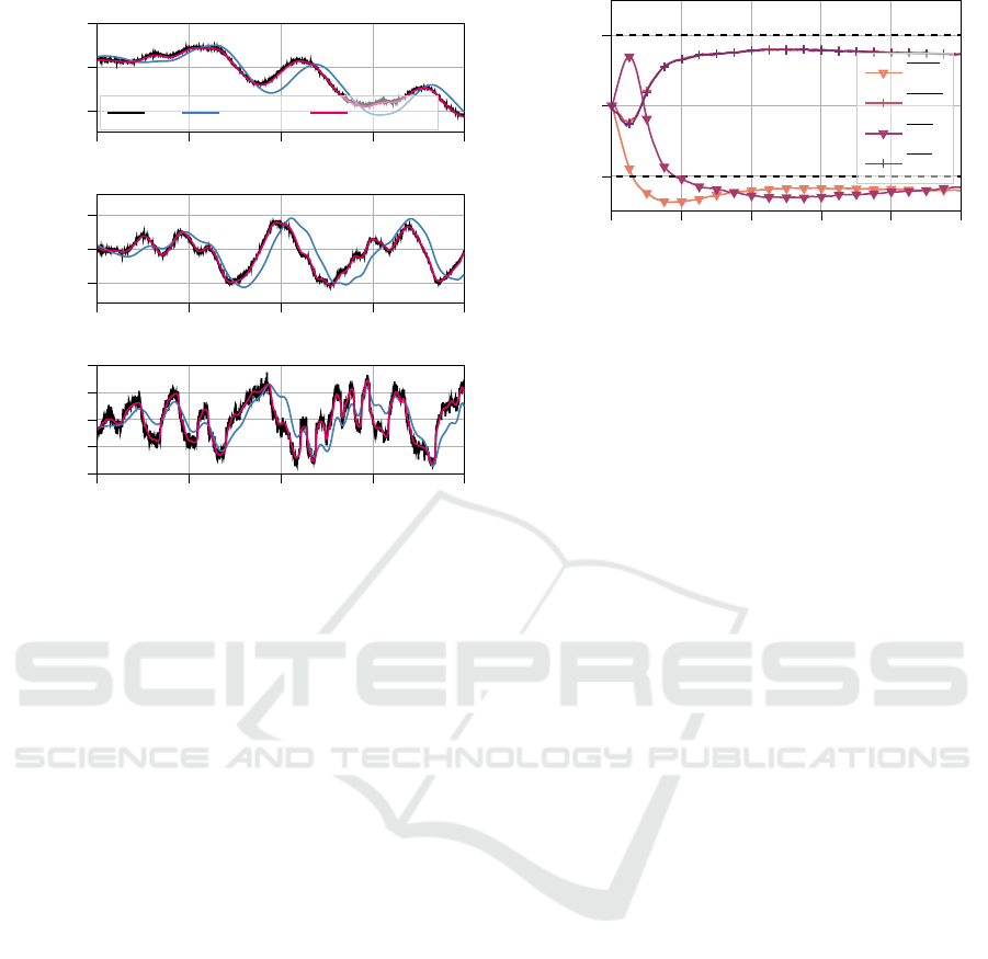
4
5 6
7 8
−2
0
2
·10
−2
z
b
(m)
ref. lin. model PeNODE
4
5 6
7 8
−5
0
5
·10
−2
v
b
(m/s)
4
5 6
7 8
−0.5
−0.25
0
0.25
0.5
Time (s)
a
b
(m/s
2
)
Figure 4: Detail of the model predictions for body-height,
-velocity and -acceleration of the linear model compared to
the trained neural ODE.
duration of one training with 1000 epochs for differ-
ent setups is measured and the results are compared
in Table 2. During the baseline training, each update
is based on the complete sequence of 42 s and the full
sample rate of 1000 Hz. In contrast, the batch updates
only use a set of 3 randomly sampled sequences, each
of 4 s length. With sub-sampling, the same settings (3
× 4 s) are used, but the loss is only calculated for 25 %
of the available points that are also randomly sampled.
The learned neural damper forces can be compared in
Figure 3a (baseline, batch, batch+subs). Additionally,
Figure 3b depicts the convergence of the loss over the
course of the training. It shows, that the learned forces
only differ slightly and the loss reaches almost the
same optimum, while mini-batching decreases the du-
ration by roughly 80 % and sub-sampling by another
30 %.
All following results were obtained with 1000
training-epochs and mini-batching as presented. Sub-
sampling was not used, since the benefit is not as sig-
nificant and the training becomes more prone to local
optima.
5.3 Model Uncertainties and Noisy Data
The previously presented results prove the princi-
ple of learning underlying non-linearities from model
output data. However, the simulated data was of high
0 200 400
600
800 1,000
−0.1
0
0.1
E poch ()
Modi f ier ()
δm
b
δm
w
δd
t
δc
t
Figure 5: Convergence of the simultaneously optimized pa-
rameter modifiers.
quality and the physical part of the hybrid model used
the nominal parameters. In the following, the robust-
ness of the approach against noisy data and model
uncertainties is investigated. To this end, the added
noise is increased by a factor of five and the parame-
ters of the neural QVM, i.e. the masses m
b
, m
w
and
the coefficients of the tire spring-damper pair c
t
and d
t
are disturbed by ± 10 % with respect to the nominal
value.
The training results under these circumstances are
included in Figure 3 (nsy+par). It shows, that the neu-
ral damper still captures the non-linear friction, with a
minor loss of precision. The same is true for the neu-
ral spring. Figure 4 gives an impression of the model
predictions before and after the training in this case,
illustrating how the learned components enhance the
model predictions despite the disturbed parameters
and presence of noise.
5.4 Simultaneous Parameter Fitting
Here we used the same setup as before (in-
creased noise, disturbed parameters) but the model-
parameters m
b
, m
w
, c
t
and d
t
are optimized alongside
the parameters of the NNs. The corresponding mod-
ifiers are saturated with γ = 0.2 as presented in Sec-
tion 2 (Eq. (7) and (8)). Figure 5 illustrates how the
modifiers converge to a near optimal value over the
course of the training. The target values for the modi-
fiers marked with plus-markers are +0.1 and the mod-
ifiers with triangles −0.1 respectively. Figure 3, lines
“nsy+par” versus “paramopt”, shows the significant
decrease of the remaining loss after the optimization
that can be attributed to the corrected model parame-
ters.
Closing the Sim-to-Real Gap with Physics-Enhanced Neural ODEs
83

6 CONCLUSIONS
In this work, we presented an approach to incorpo-
rate low-dimensional neural networks into the differ-
ential equations of a given model, forming a Physics-
enhanced Neural ODE. It showed, that missing ef-
fects are effectively learned by these neural compo-
nents, while physically meaningful behaviour can be
enforced during the training. The usage of single-
output neural networks yields the possibility to as-
sign a confidence interval to the obtained functions,
which increases the credibility of the hybrid model.
We are confident, that the presented method poses a
straightforward approach to enhance existing dynami-
cal models without sacrificing their physical integrity.
ACKNOWLEDGEMENTS
This work was organized within the European ITEA3
Call6 project UPSIM - Unleash Potentials in Simula-
tion (number 19006). The work was partially funded
by the German Federal Ministry of Education and Re-
search (BMBF, grant number 01IS20072H).
The term Physics-enhanced Neural ODEs (PeN-
ODE) was created in the proposal for the ITEA 4
project OpenSCALING.
REFERENCES
Ajay, A., Wu, J., Fazeli, N., Bauza, M., Kaelbling, L. P.,
Tenenbaum, J. B., and Rodriguez, A. (2018). Aug-
menting Physical Simulators with Stochastic Neural
Networks: Case Study of Planar Pushing and Bounc-
ing. In 2018 IEEE/RSJ International Conference on
Intelligent Robots and Systems (IROS). IEEE.
Bezanson, J., Edelman, A., Karpinski, S., and Shah, V. B.
(2017). Julia: A fresh approach to numerical comput-
ing. SIAM Review.
Bruder, F. and Mikelsons, L. (2021). Modia and Julia for
Grey Box Modeling. In Link
¨
oping Electronic Con-
ference Proceedings. Link
¨
oping University Electronic
Press.
Chang, B., Chen, M., Haber, E., and Chi, E. H. (2019). An-
tisymmetricRNN: A Dynamical System view on re-
current Neural Networks. ICLR 2019.
Chen, R. T. Q., Rubanova, Y., Bettencourt, J., and Duve-
naud, D. (2018). Neural Ordinary Differential Equa-
tions. Neural Information Processing Systems.
Daw, A., Karpatne, A., Watkins, W. D., Read, J. S.,
and Kumar, V. (2022). Physics-Guided Neural Net-
works (PGNN): An Application in Lake Temperature
Modeling. In Knowledge-Guided Machine Learning.
Chapman and Hall.
Haber, E. and Ruthotto, L. (2017). Stable Architectures for
Deep Neural Networks. Inverse Problems, Volume 34.
Heiden, E., Millard, D., Coumans, E., Sheng, Y., and
Sukhatme, G. S. (2020). NeuralSim: Augment-
ing Differentiable Simulators with Neural Networks.
IEEE International Conference on Robotics and Au-
tomation (ICRA) 2021.
Hogan, N. and Breedveld, P. (2005). The Physical Basis of
Analogies in Physical System Models. In Mechatron-
ics - An Introduction. CRC Press.
Karniadakis, G. E., Kevrekidis, I. G., Lu, L., Perdikaris,
P., Wang, S., and Yang, L. (2021). Physics-informed
Machine Learning. Nature Reviews Physics.
M
´
u
ˇ
cka, P. (2017). Simulated Road Profiles According to
ISO 8608 in Vibration Analysis. Journal of Testing
and Evaluation.
Owoyele, O. and Pal, P. (2022). ChemNODE: A neural Or-
dinary Differential Equations Framework for efficient
Chemical Dinetic Solvers. Energy and AI.
Rackauckas, C., Ma, Y., Martensen, J., Warner, C., Zubov,
K., Supekar, R., Skinner, D., Ramadhan, A., and Edel-
man, A. (2020). Universal Differential Equations for
Scientific Machine Learning.
Rai, R. and Sahu, C. K. (2020). Driven by Data or De-
rived through Physics? a Review of Hybrid Physics
Guided Machine Learning Techniques with Cyber-
Physical System (CPS) Focus. IEEE Access.
Raissi, M., Perdikaris, P., and Karniadakis, G. (2019).
Physics-Informed Neural Networks: A deep Learn-
ing Framework for Solving Forward and Inverse Prob-
lems involving nonlinear Partial Differential Equa-
tions. Journal of Computational Physics.
Ramadhan, A., Marshall, J. C., Souza, A. N., Lee, X. K.,
Piterbarg, U., Hillier, A., Wagner, G. L., Rackauckas,
C., Hill, C., Campin, J.-M., and Ferrari, R. (2022).
Capturing missing Physics in Climate Model Parame-
terizations using Neural Differential Equations. Jour-
nal of Advances in Modeling Earth Systems (JAMES).
Thummerer, T. and Mikelsons, L. (2023). Eigen-informed
NeuralODEs: Dealing with stability and convergence
issues of NeuralODEs.
Thummerer, T., Stoljar, J., and Mikelsons, L. (2022). Neu-
ralFMU: Presenting a Workflow for integrating hybrid
NeuralODEs into Real-World Applications. Electron-
ics.
Thummerer, T., Tintenherr, J., and Mikelsons, L. (2021).
Hybrid Modeling of the Human Cardiovascular Sys-
tem using NeuralFMUs. 10th International Confer-
ence on Mathematical Modeling in Physical Sciences.
Turan, E. M. and Jaschke, J. (2022). Multiple shooting for
training neural differential equations on time series.
IEEE Control Systems Letters.
Willard, J., Jia, X., Xu, S., Steinbach, M., and Kumar, V.
(2020). Integrating Physics-Based Modeling with Ma-
chine Learning: A Survey. ACM Computing Surveys.
Zeng, A., Song, S., Lee, J., Rodriguez, A., and Funkhouser,
T. (2020). TossingBot: Learning to Throw Arbitrary
Objects with Residual Physics. IEEE Transactions on
Robotics.
Zimmer, D. (2016). Equation-Based Modeling with Mod-
elica – Principles and Future Challenges. SNE Simu-
lation Notes Europe.
ICINCO 2023 - 20th International Conference on Informatics in Control, Automation and Robotics
84
