Effects Study of Sensors’ Placement on the Accuracy of a 3D

TDOA-Based Localization System

Ahcene Bellabas

1 a

, Ammar Mesloub

1 b

, Belaid Ghezali

, Abdelmadjid Maali

3 c

and Tahar Ziani

Lab. Traitement du signal, Ecole Militaire Polytechnique, BP 17 Bordj El Bahri, Algeria

Ecole Sup

erieure ALI CHABATI, Algiers, Algeria

Lab. Syst

emes

Electroniques et Num

eriques, Ecole Militaire Polytechnique, BP 17 Bordj El Bahri, Algeria

Keywords:

Passive Localization, TDOA, GDOP, Positioning.

Abstract:

Time Difference of Arrival (TDOA) based measurements are used for passive localization systems in various

applications. While signiﬁcant research has been performed on the development of TDOA measurement-

based approaches, there has been relatively little focus on the sensor deployment geometry which signiﬁcantly

impacts the location estimation accuracy. Therefore, a study on the effects of four sensors’ placement on lo-

cation accuracy has been conducted. Several factors are considered in numerical simulations analysis which

have an obvious effect on the localization accuracy. Based on the analysis of the Geometric Dilution of Preci-

sion (GDOP) performance metric, a comparison is conducted between square and star geometries. The results

show that the star geometry gives better performance in terms of location estimation accuracy, especially when

the main receiver is positioned within the polygon formed with baseline angles of 120°. Furthermore, the star

geometry is used to study also the inﬂuence of sensor height and baseline length to achieve an optimum three-

dimensional sensor placement with four sensors. The results can be applied to enhance the sensor deployment

in 3D sensor geometry for TDOA-based localization systems.

1 INTRODUCTION

Recently, passive localization systems have assumed

a signiﬁcant role in various civilian and military appli-

cations, including radar, sonar and navigation. These

systems commonly employ time measurement-based

localization techniques, which can be classiﬁed as fol-

lows: Time of Arrival (TOA) and TDOA, also known

as multilateration technique (Wan et al., 2018; Deng

et al., 2019). The later use TDOA measurements ob-

served at a set of spatially separated receivers. Each

TDOA measurement deﬁnes a hyperbolic line, and

the intersection of these lines gives the estimation of

the source location.

The literature has mainly focused on develop-

ing TDOA measurements-based approaches to im-

prove location estimation accuracy. Other works have

aimed to enhance localization performance in terms

of location estimation accuracy, which depends on

various factors such as the number of sensor used,

https://orcid.org/0000-0002-2375-5364

https://orcid.org/0000-0002-3754-8382

https://orcid.org/0000-0003-3652-1943

the choice of main or reference sensor used to gener-

ate the TDOA measurements, the multilateration ap-

proach, and sensor deployment geometry (Sun et al.,

2016; Shehu and Sha’ameri, 2018a; Shehu, 2018).

Although the latter factor signiﬁcantly inﬂuences the

location estimation accuracy, little research, as far as

we know, has been conducted on it, as works pre-

sented in (Qin et al., 2016; Shehu and Sha’ameri,

2018b). Therefore, in order to enhance localization

performance, it is necessary to investigate the optimal

geometry.

In this paper, we focus on studying the impact of

four sensors’ deployment geometry on the location

performance using TDOA measurements. Speciﬁ-

cally, two geometries, namely square and star geome-

try, are evaluated to determine the optimal choice for

location estimation accuracy. The selected geometry

is then used to investigate the inﬂuence of other fac-

tors, namely baseline angle, sensor height and base-

line length. In this context, a baseline refers to the

line connecting the main sensor and one of the three

auxiliary sensors. The analysis of the GDOP parame-

ter (Li et al., 2011; Thompson et al., 2019) forms the

basis of this study, enabling a comprehensive assess-

Bellabas, A., Mesloub, A., Ghezali, B., Maali, A. and Ziani, T.

Effects Study of Sensors’ Placement on the Accuracy of a 3D TDOA-Based Localization System.

DOI: 10.5220/0012161600003543

In Proceedings of the 20th International Conference on Informatics in Control, Automation and Robotics (ICINCO 2023) - Volume 2, pages 94-100

ISBN: 978-989-758-670-5; ISSN: 2184-2809

ment of the localization system’s performance under

varying deployment geometries.

The remainder of the paper is organized as fol-

lows: the location system geometry is described in

section 2, the hyperbolic position location (PL) ap-

proach and its theoretical model are shown in section

3, the theoretical derivation of the GDOP is given in

section 4, the simulation result and discussion are de-

tailed in section 5, which is followed by conclusion in

section 6.

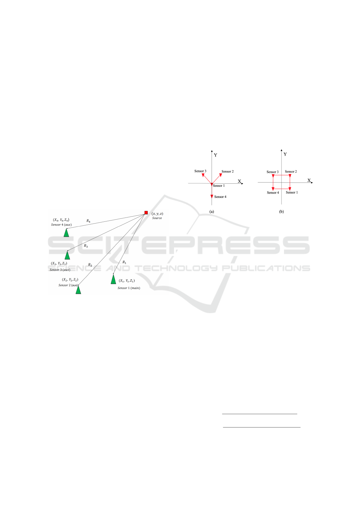
2 SYSTEM GEOMETRY

Let us consider the scenario illustrated in Figure 1,

which presents a system geometry for TDOA-based

location consisting of four sensors (receivers). We set

sensor 1 as the main receiver and set others as the

auxiliary receivers. Let us consider (X

, Y

, Z

) the po-

sition coordinates of the sensor i, for i = 1, ..., 4. The

source is on the position (x, y, z).

Figure 1: System geometry considered for TDOA based lo-

calization.

The localization accuracy is dependent on the de-

ployment of the sensors, which can be character-

ized by the GDOP or the Cramer-Rao Lower Band

(CRLB) (Vankayalapati, 2014; Li et al., 2017; Zhang

and Lu, 2020; Diez-Gonzalez et al., 2020; Wang

et al., 2022). The CRLB is a concept widely used in

positioning performance analysis. It determines the

minimum achievable error of a locating system with

independence from the positioning algorithm used

(

Alvarez et al., 2019).

In this work, the average values of GDOP for dif-

ferent sensors’ deployment geometries are examined

for optimization in a 3D TDOA-based location sys-

tem. The following steps are taken

• Two geometries are chosen to deploy the four sen-

sors, named star and square geometry (Figure 2).

• The geometry that will give the best localization

performance will be selected to study the inﬂu-

ence of other factors on localization performance.

• The factors that will be studied are the baseline

angle, heights of the four sensors and baseline

length.

The subsequent sections of this paper cover two

main aspects. Firstly, we describe the hyperbolic po-

sition location system, followed by the development

of its GDOP to analyze the optimal sensors’ deploy-

ment geometry. Lastly, we present simulation results

that evaluate the TDOA localization performance for

various geometries.

Figure 2: Geometries considered for evaluation. (a) star

geometry. (b) square geometry.

3 HYPERBOLIC PL SYSTEM

TDOA measurements can be used to localize a target

(source). Its location is estimated by the intersection

of hyperboloids describing range difference measure-

ments between three or more sensors. The foci of the

hyperboloid are at the positions of the sensors i and j.

In a system with N sensors, there are N −1 linearly in-

dependent TDOA measurements. The geometric ap-

proach uses intersecting hyperboloid surfaces created

from the TDOA measurements made by the passive

sensors to determine the target location (Wong et al.,

2017).

The relationship between the Range Difference of

Arrival (RDOA) and TDOA, is given by

i, j

= c τ

i, j

= R

− R

(1)

where R

and R

, are the distances from the source

to the sensors i, j respectively, R

i, j

and τ

i, j

are the

RDOA and TDOA of a signal received by sensor pair

i and j and c is signal propagation speed.

In a three-dimensional (3D) system, the hyper-

boloids that describe the range difference, R

i, j

be-

tween sensor positions are given by

i, j

− x)

+ (Y

− y)

+ (Z

− z)

−

− x)

+ (Y

− y)

+ (Z

− z)

(2)

Effects Study of Sensors’ Placement on the Accuracy of a 3D TDOA-Based Localization System

where: (X

, Y

, Z

) and (X

, Y

, Z

) deﬁne the positions

of sensor i and j respectively, and (x, y, z) is the source

position.

The TDOA method offers a signiﬁcant beneﬁt as it

does not require knowledge of the transmit time from

the source, eliminating the need for strict clock syn-

chronization between the source and receiver (Wang

et al., 2019). Furthermore, unlike TOA methods, the

hyperbolic position location method can reduce or

eliminate common errors experienced at all sensors

due to the channel.

Referring all TDOAs to the main sensor, which is

assumed to be the reference for all sensors, let us use

’i’ with i = 2, ..., M to represent the auxiliary sensors.

The range difference between sensors with respect to

the main sensor, is

i,1

= cτ

i,1

= R

− R

− x)

+ (Y

− y)

+ (Z

− z)

−

− x)

+ (Y

− y)

+ (Z

− z)

(3)

where, R

i,1

and τ

i,1

are the range and time difference

measurements between the main sensor and the i

sensor, and R

is the distance from the main sensor

to the source. This deﬁnes the set of nonlinear hyper-

bolic equations whose solution gives the 3D source

location. Numerical methods are needed to solve

the nonlinear equations of (3) (D

ıez-Gonz

alez et al.,

2022). Linearizing this set of equations is commonly

performed using typical TDOA location algorithms

which are: the Chan algorithm, Fang algorithm, and

Taylor series expansion algorithm (Foy, 1976; Chan

and Ho, 1994; Zhang and TAN, 2008; Al Harbi and

Helgert, 2010). Fang algorithm and Chan algorithm

are closed-form algorithms with analytic expressions.

Taylor series expansion algorithm is an iterative algo-

rithm without analytic expression.

4 GDOP FOR TDOA BASED

LOCALIZATION

GDOP is a metric used to describe the effect of geom-

etry on the relationship between the measurement and

position error. It is a measure of the quality of the ge-

ometric conﬁguration of the sensor array and is used

to evaluate the accuracy of TDOA-based localization

systems (Elgamoudi et al., 2021). The lower the

GDOP, the better the geometric conﬁguration. The

optimal placement of the sensors is the one that mini-

mizes the GDOP.

A range measurement can be expressed as

L = f (x, y, z) (4)

where L is a measured value, and (x, y, z) are unknown

coordinates of the source. We use the Taylor series

expansion algorithm to linearize the equation (4) by

developing the function f (x, y, z) to the ﬁrst order

L ≈ f (x

, y

, z

) +

(

∂L

∂x

)

(

∂L

∂y

)

(

∂L

∂z

)

(5)

where (x

, y

, z

) is the initial estimation of the source

coordinates, and (

∂L

∂x

)

, (

∂L

∂y

)

, and (

∂L

∂z

)

are the par-

tial derivatives of the measured value L evaluated at

the initial estimation.

Assume there are n observations, equation (5) can

be written in the following matrix form

H∆x = ∆r (6)

∆x = (H

−1

∆r (7)

where ∆x is the vector offset of the true source posi-

tion from the linearization point, ∆r is the vector off-

set of the true range to the range values corresponding

to the linearization point, and H is a matrix that can

be presented as

H =







(

∂L

∂x

)

(

∂L

∂y

)

(

∂L

∂z

)

(

∂L

∂x

)

(

∂L

∂y

)

(

∂L

∂z

)

(

∂L

∂x

)

(

∂L

∂y

)

(

∂L

∂z

)







(8)

In the case of hyperbolic multilateration system,

the measured values are TDOAs, so

L = R

i,1

− x)

+ (Y

− y)

+ (Z

− z)

−

− x)

+ (Y

− y)

+ (Z

− z)

(9)

with : i = 2, ..., M.

As previously mentioned, the considered TDOA

multilateration positioning system consists of a main

and three auxiliary sensors (M = 4). After calculat-

ing the various partial derivatives, matrix H can be

expressed as

H =







− X

−

− X

−Y

−

−Y

− Z

−

− Z

− X

−

− X

−Y

−

−Y

− Z

−

− Z

− X

−

− X

−Y

−

−Y

− Z

−

− Z







(10)

GDOP is deﬁned as the ratio of the Root Mean

Square (RMS) position error to the RMS ranging er-

ror (Elgamoudi et al., 2021)

GDOP =

+ σ

(11)

ICINCO 2023 - 20th International Conference on Informatics in Control, Automation and Robotics

with σ

the variance of the measurement error on the

range.

The provided mathematical expression for GDOP

is a general form applicable to various scenarios. In

the following discussion, we will speciﬁcally derive

an explicit expression for GDOP in the context of a

TDOA location system with four receivers.

Assuming the errors in the measurements on the

range are random, independent, have zero mean, and

an identical rms σ

. The estimated distance is

= R

+ dr

, j = 1, ..., 4 (12)

By performing the necessary calculations, we can de-

termine the variances and covariances of the errors on

range differences. The outcome of this calculation is

presented in the subsequent error covariance matrix

for RDOA

Q = σ







2 1 ··· 1

1 2 ··· 1

1 1 1 2







(13)

The covariance of ∆x is calculated by using equation

(7) as follows

cov(∆x) = E[∆x∆x

]

= E[(H

−1

∆r∆r

H(H

−1

]

= H

−1

)

−1

QHH

−1

)

−1

= H

−1

Q(H

)

−1

= (H

−1

(14)

Finally, the expression for GDOP is presented as fol-

lows

GDOP =

+ σ

∑

i=1

((H

−1

)

i,i

(15)

The GDOP can be obtained by deriving it from

the CRLB in the following manner (Thompson et al.,

2019):

GDOP =

trace(CRLB(P)) (16)

where P is the source position (x, y, z).

5 SIMULATION AND ANALYSIS

We consider the depicted location system geometry

in Figure 1 for our analysis. The area of interest is

a surface [200 × 200] Km

, in which we calculate the

GDOP for a target at a height of 7000 m. The sen-

sor coordinates (X

, Y

, Z

), i ∈ 1, . . . 4 are chosen as

follows for the square geometry: {(0, 0, 0), (20, 0, 0),

(20, 20, 0), and (0, 20, 0)} Km. Similarly, for the

star geometry, the sensor coordinates are selected

as:{(0, 0, 0),(20, 0, 0), (−20, −20, 0), and (0, 20, 0)}

Km.

The measurement noise was assumed to be Gaus-

sian white with zero mean and standard deviation

(RMS ranging error) σ

= 1 m.

The results of the GDOP calculation for the two

sensor conﬁgurations, square and star geometry, are

depicted in Figures 3 and 4, respectively. The values

are presented in meters.

Figure 3: 3D GDOP calculation for square geometry.

Figure 4: 3D GDOP calculation for star geometry.

To ensure meaningful calculations, in cases where

the GDOP value at a speciﬁc location is excessively

large or cannot be calculated, a value of 300 is as-

signed.

These simulation results indicate that the positions

of the sensors has a direct impact on the performance

of localization, since changing their positions leads to

varying GDOP values. Thus, the deployment geome-

try of the sensors directly inﬂuences the performance

Effects Study of Sensors’ Placement on the Accuracy of a 3D TDOA-Based Localization System

of localization. From the former, it can be seen clairly

that the star geometry outperforms the square geome-

try in terms of performance.

These results reveal some intriguing observations.

Firstly, it is evident that the GDOP is notably higher

(worse) at the center of the square conﬁguration. This

ﬁnding aligns with the report of (Li et al., 2011),

which highlights that deploying the base stations (sen-

sors) exclusively along the perimeter of an area leads

to poor DOP at the center of the polygon. Sec-

ondly, in the square geometry, a notable degradation

in GDOP occurs when moving along the direction of

the square’s medians beyond the receiver’s area (as

depicted in Figure 3). Consequently, this conﬁgu-

ration is unsuitable for target localization due to the

substantial ambiguity zone it presents.

Finally, in the scenario of the star geometry, the

localization accuracy exhibits a consistent pattern as

one moves farther from the sensors. Additionally, the

GDOP remains good within the inner region encom-

passing the receiver positions and the surrounding

area. For instance, when aiming for a tolerated local-

ization error of less than 100 m, the location system

covers a contiguous area exceeding [100 × 100] Km

The star geometry can be achieved by moving one

of the sensors to the center of the square geometry.

Consequently, placing a receiver at the center of a

polygon enhances the GDOP within the sensor’s area.

Therefore, this geometry will be utilized in subse-

quent analyses to study the impact of various factors

on localization performance. These factors include

the baseline angle, heights of the four sensors, and

baseline length.

5.1 Effect of Baseline Angle

Let us consider the sensor deployment geometry de-

picted in Figure 5. The coordinates of the four sensors

are as follows

, Y

, Z

) = (0, 0, 0)(m)

, Y

, Z

) = (R × sin(θ

), −R × cos(θ

), 0)(m)

, Y

, Z

) = (−R × sin(θ

), −R × cos(θ

), 0)(m)

, Y

, Z

) = (0, −R, 0)(m)

The RMS ranging error and the baseline length are set

to ﬁxed values: σ

= 0.2 m, R = 20 × 10

To investigate the impact of baseline angles, θ

and θ

, we conducted a comprehensive analysis by

varying their values within the range of 15° to 165°.

For each conﬁguration, the average GDOP was com-

puted over the designated area of interest. The results

obtained from the simulations are presented in Figure

Figure 5: The selected geometry to study the effect of base-

line angle.

GDOP average

101

104

107

110

113

116

119

122

125

128

131

134

137

140

143

146

149

152

155

158

20 40 60 80 100 120 140 160

Angle

100

120

140

160

Angle

100

120

140

160

180

200

Figure 6: Effect of baseline angles variation on location per-

formances. Angles are provided in degrees.

It is worth noting that the deployment geome-

try of the receivers signiﬁcantly affects the perfor-

mance of localization. Based on the obtained results,

the optimal conﬁguration is characterized by angles

of 120° between the different baselines [RS

− RS

[RS

− RS

], and [RS

− RS

]. This particular conﬁg-

uration exhibits the lowest average GDOP.

5.2 Effect of Sensor Height

In this scenario, we focus on the optimal sensors’ de-

ployment geometry obtained in the previous subsec-

tion 5.1, where the baseline angles were set at θ=120°.

We now proceed to vary the height of the main sensor

while keeping heights of the other sensors (auxiliary)

at a ﬁxed level. Similarly to previous simulations, we

calculate the average GDOP for each conﬁguration.

The results are presented in Figure 7.

We observe that the larger the difference between

the height of the reference sensor and that of the other

sensors, the more the localization performance is de-

graded (Figure 7). Therefore, the height of the main

sensor in a TDOA-based localization system should

be close to that of the other sensors to achieve better

localization.

ICINCO 2023 - 20th International Conference on Informatics in Control, Automation and Robotics

0 200 400 600 800 1000

Main sensor height (m)

GDOP average

Figure 7: Effect of the main sensor height on location per-

formances.

Now, let us explore the effect of changing the

height of an auxliary sensor on the localization per-

formance.

0 200 400 600 800 1000

Auxiliary sensor height (m)

GDOP average

Sensor 2 (aux)

Sensor 3 (aux)

Sensor 4 (aux)

Figure 8: Effect of auxiliary sensor height on location per-

formances.

When we keep the height of the main sensor ﬁxed

and vary the heights of the remaining sensors one

by one, we observe that it has minimal impact on

the localization performance (Figure 8). The values

of GDOP remain practically stable throughout these

variations. This indicates that the height of individ-

ual auxiliary sensors does not signiﬁcantly impact the

overall localization system performance.

5.3 Effect of Baseline Length

The baseline lenght is another factor to consider in

evaluating the performance of TDOA-based localiza-

tion. Its impact is investigated by variying the length

of the three baselines in the same way, examining its

effect on the GDOP values. It is important to note that

the deployment geometry remains the same (star ge-

ometry with baseline angle θ=120°) throughout this

analysis. The simulation results are presented in Fig-

ure 9. The values are presented in meters.

It is observed that lengthening baseline length

leads to improved localization accuracy. This im-

provement can be attributed to the larger TDOA val-

ues obtained with greater distances, leading to en-

0 2 4 6 8 10

Baseline length (m)

GDOP average

Figure 9: Inﬂuence of baseline length variation on location

performances.

hanced accuracy in the estimation of the source’s lo-

cation. However, it is important to note that there is a

limit to increasing the baseline length as it can lead to

a potential risk of signal detection failure by the sen-

sors, where the emitted signal from the source may

not be detected by a sensor. In such cases, with fewer

available equations, it becomes challenging to accu-

rately locate the source. Therefore, careful consider-

ation must be given to strike a balance between max-

imizing baseline length for improved accuracy while

ensuring reliable signal detection and localization.

6 CONCLUSION

This paper focuses on the optimization of sensor

deployment in a 3D TDOA-based location system.

GDOP is used as a performance metric to evaluate

localization performance. The GDOP for a TDOA

location system with four sensors is derived and an-

alyzed. It is shown that the deployment geometry of

the sensors directly impacts localization performance.

A comparison was ﬁrst made between a square geom-

etry and a star geometry. The latter was efﬁcient and

its localization accuracy exhibits a consistent pattern

as one moves farther from the sensors. Thus, the star

geometry was selected to investigate the inﬂuence of

other factors on localization performance, namely :

the baseline angle, sensor height, and baseline length.

It is found that a sensor deployment conﬁguration

with baseline angles of 120° gives optimal results. As

for the impact of sensor height, only changes in the

main sensor height signiﬁcantly affect localization er-

rors, as it serves as the reference in TDOA methods.

Finally, increasing the baseline length enhances loca-

tion accuracy. Future research should focus on formu-

lating an optimization problem for sensor deployment

and proposing algorithms to design an optimal strat-

egy. The effectiveness of the strategy should also be

Effects Study of Sensors’ Placement on the Accuracy of a 3D TDOA-Based Localization System

evaluated.

REFERENCES

Al Harbi, F. S. and Helgert, H. J. (2010). An improved chan-

ho location algorithm for tdoa subscriber position es-

timation. International journal of computer science

and network security, 10(9):101–105.

Alvarez, R., D

ıez-Gonz

alez, J., Alonso, E., Fern

andez-

Robles, L., Castej

on-Limas, M., and Perez, H. (2019).

Accuracy analysis in sensor networks for asyn-

chronous positioning methods. Sensors, 19(13):3024.

Chan, Y. and Ho, K. (1994). A simple and efﬁcient esti-

mator for hyperbolic location. IEEE Transactions on

Signal Processing, 42:1905 – 1915.

Deng, Z., Wang, H., Zheng, X., Fu, X., Yin, L., Tang, S.,

and Yang, F. (2019). A closed-form localization al-

gorithm and gdop analysis for multiple tdoas and sin-

gle toa based hybrid positioning. Applied Sciences,

9(22):4935.

Diez-Gonzalez, J., Alvarez, R., Prieto-Fernandez, N., and

Perez, H. (2020). Local wireless sensor networks

positioning reliability under sensor failure. Sensors,

20(5):1426.

ıez-Gonz

alez, J.,

Alvarez, R., Verde, P., Ferrero-Guill

en,

R., and Perez, H. (2022). Analysis of reliable deploy-

ment of tdoa local positioning architectures. Neuro-

computing, 484:149–160.

Elgamoudi, A., Benzerrouk, H., Elango, G. A., and

Landry Jr, R. (2021). A survey for recent tech-

niques and algorithms of geolocation and target track-

ing in wireless and satellite systems. Applied Sciences,

11(13):6079.

Foy, W. H. (1976). Position-location solutions by taylor-

series estimation. IEEE transactions on aerospace

and electronic systems, (2):187–194.

Li, B., Dempster, A., and Wang, J. (2011). 3D DOPs for

positioning applications using range measurements.

Wireless Sensor Network, 3:343–349.

Li, W., Yuan, T., Wang, B., Tang, Q., Li, Y., and Liao,

H. (2017). Gdop and the crb for positioning sys-

tems. IEICE Transactions on Fundamentals of Elec-

tronics, Communications and Computer Sciences,

100(2):733–737.

Qin, Z., Wang, J., and Wei, S. (2016). A study of 3d sensor

array geometry for tdoa based localization. In 2016

CIE International Conference on Radar (RADAR),

pages 1–5. IEEE.

Shehu, Y. (2018). Position estimation performance eval-

uation of a linear lateration algorithm with an SNR-

based reference station selection technique. Nigerian

Journal of Technology, 34.

Shehu, Y. and Sha’ameri, A. (2018a). Closed-form 3-D

position estimation lateration algorithm reference pair

selection technique for a multilateration system. Jour-

nal of Telecommunication, 10.

Shehu, Y. and Sha’ameri, A. (2018b). Effect of path loss

propagation model on the position estimation accu-

racy of a 3-dimensional minimum conﬁguration mul-

tilateration system. International Journal of Inte-

grated Engineering, 10:35–42.

Sun, S., Wang, Z., and Wang, Z. (2016). Study on opti-

mal station distribution based on tdoa measurements.

In 2016 International Conference on Computer Engi-

neering, Information Science & Application Technol-

ogy (ICCIA 2016), pages 283–288. Atlantis Press.

Thompson, R., Balaei, A., and Dempster, A. (2019). Di-

lution of precision for GNSS interference localisation

systems.

Vankayalapati, Naresh; Kay, S. Q. D. (2014). TDOA

based direct positioning maximum likelihood estima-

tor and the cramer-rao bound. IEEE Transactions on

Aerospace and Electronic Systems, 50.

Wan, P., Ni, Y., Hao, B., Li, Z., and Zhao, Y. (2018). Passive

localization of signal source based on wireless sen-

sor network in the air. International Journal of Dis-

tributed Sensor Networks, 14(3):1550147718767371.

Wang, D., Yin, J., Chen, X., Jia, C., and Wei, F. (2019). On

the use of calibration emitters for tdoa source localiza-

tion in the presence of synchronization clock bias and

sensor location errors. EURASIP Journal on Advances

in Signal Processing, 2019(1):1–34.

Wang, Y., Zhou, T., Yi, W., and Kong, L. (2022). A gdop-

based performance description of toa localization with

uncertain measurements. Remote Sensing, 14(4):910.

Wong, S., Jassemi-Zargani, R., Brookes, D., and Kim, B.

(2017). A geometric approach to passive target local-

ization. S&T Organization.

Zhang, J. and Lu, J. (2020). Analytical evaluation of ge-

ometric dilution of precision for three-dimensional

angle-of-arrival target localization in wireless sensor

networks. International Journal of Distributed Sensor

Networks, 16(5):1550147720920471.

Zhang, L. and TAN, Z. (2008). A new TDOA algorithm

based on Taylor series expansion in cellular networks.

Frontiers of Electrical and Electronic Engineering in

China, SP Higher Education Press.

ICINCO 2023 - 20th International Conference on Informatics in Control, Automation and Robotics

100