Experimental Validation of the Non-Orthogonal Serret–Frenet

Parametrization Applied to the Path Following Task

Filip Dyba

Department of Cybernetics and Robotics, Faculty of Electronics, Photonics and Microsystems,

Wrocław University of Science and Technology, Janiszewskiego Street 11/17, Wrocław, 50-372, Poland

ﬁ

Keywords:

Backstepping Integrator, KINOVA

Redundant Manipulator, Non-Orthogonal Projection, Path Following,

Serret–Frenet Parametrization.

Abstract:

The path following task belongs to the fundamental robotic tasks. It consists of following a spatial curve

parametrized with a curvilinear distance. In this time-independent approach no time regimes are imposed

on a robot. In fact, it is a natural deﬁnition of a task for many robots, e.g. autonomous vehicles. In the

paper a path following algorithm based on the non-orthogonal Serret–Frenet parametrization is presented.

Such an approach is global and does not introduce any constraints to the robot description with respect to

the path. It has been extensively studied recently. Hence, an experimental veriﬁcation of the algorithm is

proposed. The validation was conducted on a laboratory test–bed equipped with a redundant manipulator —

the KINOVA

Gen3 Ultra lightweight robot. In the paper a case study is proposed to compare simulation

results and experimental measurements. It is an example how the mathematical legacy of the past centuries

can be used for modern solutions. The experimental study conﬁrms the practical suitability of the presented

control algorithm.

1 INTRODUCTION

The path following task is one of the basic robotic

tasks distinguished in the literature and is a common

task in many contemporary applications. It seems

to be a natural solution to the encountered prob-

lems in modern robotics, e.g. it is eagerly used to

control autonomous vehicles (Rokonuzzaman et al.,

2021; Encarnac¸

ao and Pascoal, 2000). Moreover, re-

searchers have successfully harnessed the idea of path

tracking for some non-obvious applications, such as

controlling ﬂying robots (Lugo-C

ardenas et al., 2017)

or mobile manipulators (Mazur and Szakiel, 2009).

Hence, in the paper the next step in the development

of the path following algorithms, namely the experi-

mental validation, is presented.

According to (Hung et al., 2023), the task is to

force a robot to approach and move along a geomet-

rical curve (path) deﬁned in its workspace, whereas

a velocity proﬁle along the path has to be asymptoti-

cally tracked. A path is a purely geometrical descrip-

tion of a motion. It means that no time regimes are im-

posed on a controlled robot. The lack of time depen-

https://orcid.org/0000-0001-9202-519X

dency is particularly vital in applications with con-

trol constraints. It is a clear advantage in comparison

with some time-dependent approaches, such as the

trajectory tracking problem (Mazur and Cholewi

nski,

2016).

In the literature different approaches to the path

description can be met, namely the parametric meth-

ods (Mazur and Płaskonka, 2012; Liao et al., 2015)

and the non-parametric techniques (Morro et al.,

2011; Michałek and Gawron, 2018). The ﬁrst ap-

proach is focused on a geometrical description of

a robot with respect to a moving reference object,

while the second one is a purely numerical analy-

sis of shapes and surfaces. In the paper the para-

metric approach is experimentally veriﬁed as it has

been eagerly considered in many applications, both

on the plane (Micaelli and Samson, 1993; Płaskonka,

2013; Domski and Mazur, 2018) and in the three-

dimensional space (Mazur et al., 2015; Cholewi

nski

and Mazur, 2019).

The most frequently considered curvilin-

ear parametrization method is the Serret–Frenet

parametrization. It allows one to describe a robot

with respect to a curve. In order to do so, a robot’s

guidance point needs to be projected onto the path.

608

Dyba, F.

Experimental Validation of the Non-Orthogonal Serret-Frenet Parametrization Applied to the Path Following Task.

DOI: 10.5220/0012164200003543

In Proceedings of the 20th International Conference on Informatics in Control, Automation and Robotics (ICINCO 2023) - Volume 1, pages 608-615

ISBN: 978-989-758-670-5; ISSN: 2184-2809

Two approaches are distinguished: orthogonal and

non-orthogonal. The orthogonal projection (Dyba

and Mazur, 2023) is valid only locally and requires

ﬁnding the shortest distance between the controlled

robot and the path. In contrary, the non-orthogonal

projection is a global method. Although it requires

considering more control variables, it does not

introduce any additional constraints.

Due to that facts, the non-orthogonal Serret–

Frenet parametrization has been intensively investi-

gated (Mazur and Dyba, 2023). The algorithm has

been designed with the usage of the backstepping in-

tegrator method (Krsti

c et al., 1995), because of the

cascaded structure of the system.

In the paper an experimental validation of the

theoretically designed algorithm is presented. The

simulation study is validated with experiments on

a test–bed consisting of the KINOVA

Gen3 Ultra

lightweight robot. The gathered measurements are

compared in order to evaluate the practical usefulness

of the proposed control algorithm.

2 Serret–Frenet

PARAMETRIZATION

The most popular curvilinear parametrization was de-

ﬁned in 19

century by Serret and Frenet. It is ea-

gerly used in many contemporary applications in var-

ious ﬁelds such as mathematics, physics, computer

graphics and also in robotics. This parametric de-

scription of a curve deﬁnes a local frame consisting

of three unit vectors: tangent to a curve T , normal to

a curve N , and binormal to a curve B. They span

an orthonormal basis in R

. The Serret–Frenet frame,

which is also frequently called the Frenet trihedron,

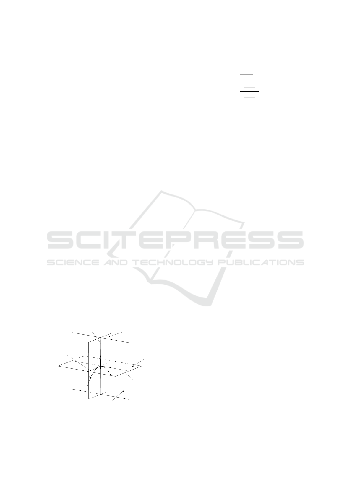
describes the curve geometry locally. Its visualization

is presented in Fig. 1. The base vectors of the Serret–

normal plane

main normal

straightening

plane

strictly tangent

plane

binormal

tangent

r(s)

Figure 1: Frenet trihedron.

Frenet frame are deﬁned as follows (Oprea, 2007)

T (s) =

dr(s)

, (1a)

N (s) =

dT (s)



dT (s)



, (1b)

B(s) = T (s) ×N (s), (1c)

where r(s) is the analytical description of a curve

in R

, and s is the so-called curvilinear distance. The

s parameter should be understood as the distance from

the assumed initial point of a curve to the current

point. Its value is equal to the length of a string placed

precisely along a curve (Dyba and Mazur, 2023).

The evolution of the Serret–Frenet frame fully de-

scribes the geometry of a curve. Let us deﬁne a ro-

tation matrix which consists of base vectors spanning

Frenet trihedron, i.e.

S(s) =



T (s) N(s) B(s)



, (2)

S ∈ SO(3) (Selig, 2005). Then, the frame evolution

is expressed with the equation (Oprea, 2007)

dS(s)





(s)









0 −κ(s) 0

κ(s) 0 −τ(s)

0 τ(s) 0





= S(s)W (s), (3)

where κ is the curvature (the curve swerve from

a straight line), τ is the torsion (the curve swerve

from a plane), and W is the antisymmetric matrix,

i.e. W = −W

. It should be emphasized that the

frame evolution directly depends on the geometrical

invariants κ and τ, which are deﬁned as (Mazur et al.,

2015)

κ(s) =



dT (s)



, (4a)

τ(s) =

(s)



dr(s)

r(s)



, (4b)

where ⟨·,·⟩ denotes a scalar product of vectors.

3 MATHEMATICAL MODEL OF

A ROBOT

In the paper a holonomic stationary manipulator is

taken into account. It is assumed that it is a redun-

dant robot. Hence, it has more than six degrees of

freedom, i.e. q ∈ R

, n > 6, where q is the vector of

the manipulator conﬁguration consisting of joint po-

sitions.

Experimental Validation of the Non-Orthogonal Serret-Frenet Parametrization Applied to the Path Following Task

609

The position of the end-effector in the base frame

may be calculated according to the forward kinemat-

ics task (Spong and Vidyasagar, 1991)

p = k(q ) ∈R

. (5)

The position p will be referred to as the robot guid-

ance point. The end-effector velocities may be calcu-

lated from the equation



˙p



= J(q) ˙q =



(q)



˙q, (6)

where ˙p is the linear velocity of the end-effector, ω is

its angular velocity, and J (q) ∈ R

6×n

is the Jacobi

matrix which consists of submatrices J

∈ R

3×n

corresponding to transformations to linear and angu-

lar velocities, respectively. In the following sections

only the end-effector position and its linear velocity

will be considered. Hence, let us deﬁne the matrix J

(q) =

∂k(q)

∂q

. (7)

Dynamics of the manipulator is derived with

the usage of the Lagrange formalism (Siciliano and

Khatib, 2007) and the model is expressed as

M (q) ¨q + C( ˙q,q) ˙q + D(q) = u, (8)

where M (q) ∈ R

n×n

deﬁnes the inertia matrix,

C( ˙q,q) ∈R

n×n

is the matrix of Coriolis and centrifu-

gal forces, D(q) ∈ R

is the vector of gravity terms,

and u ∈R

denotes the generalized control forces ap-

plied to respective joints. In the model (8) other dy-

namics effects, such as friction, are neglected.

3.1 Robot Equations with Respect

to a Path

In order to describe a robot with respect to a path,

understood as a curve in R

space, the robot guid-

ance point P has to be projected onto the path. To do

so, the non-orthogonal projection may be harnessed.

Such a method is a global procedure and it does not

introduce any singularities in the robot description.

The point projected onto a path P

′

may be at any dis-

tance from the guidance point P, i.e. it may be located

ahead of the point P or behind it during the robot mo-

tion. The point P

′

is at a distance s from the initial

point of the curve, so it is also the origin point of

the Serret–Frenet frame associated with the path. The

idea of the non-orthogonal projection is presented in

Fig. 2. The X

frame is the global reference frame

which is identiﬁed with the manipulator base frame.

According to the notation in Fig. 2, the position

of the robot guidance point with respect to the local

Serret–Frenet frame is deﬁned as

d = S

(p −r) =





. (9)

′

Figure 2: Non-orthogonal projection of the robot guidance

point P onto the curve r.

The robot kinematics with respect to the path is

derived by differentiating equation (9)

d = S

( ˙p − ˙r) +

(p −r). (10)

Let us notice that the element S

˙r deﬁnes the linear

velocity of the point P

′

in the Serret–Frenet reference

frame. Hence, the following relation holds

˙r =







T ,





N ,











˙s

(1a)





˙s





. (11)

Moreover, it is true that

(p −r) = ˙s

(p −r)

(3)

= ˙s (SW )

(p −r) =

= −˙sW S

(p −r)

(9)

= −˙sW d. (12)

As a result, equation (10) is reformulated taking into

account equations (6), (11) and (12)

d = S

˙q −





˙s





− ˙sW d = L ˙q + F , (13)

where L = S

∈ R

3×n

, and F ∈ R

4 CONTROL PROBLEM

FORMULATION

The control problem is to enforce the motion of the

manipulator end-effector along a spatial path deﬁned

in the robot workspace.

The following assumptions are made:

ICINCO 2023 - 20th International Conference on Informatics in Control, Automation and Robotics

610

• the desired path is deﬁned as a pure geometrical

object in R

space;

• the Serret–Frenet frame is well-deﬁned in every

point of the path, so the curve is at least of C

class and has no zero-curvature points;

• the desired velocity proﬁle of the Serret–Frenet

frame along the path is deﬁned arbitrarily and

tracked during the manipulator motion;

• the considered manipulator is stationary, holo-

nomic and redundant;

• the manipulator kinematics is precisely known

and the robot operates outside the singular con-

ﬁgurations;

• parameters of the manipulator dynamics may re-

main unknown;

• only control of the end-effector position is consid-

ered.

It is worth noticing that tracking of the desired veloc-

ity proﬁle along the path is a secondary subproblem.

The proﬁle deﬁnes the motion of the Serret–Frenet

frame and does not violate the geometrical descrip-

tion of the path. It may be freely tuned regarding the

robot limitations.

It may be observed that the full model of the ma-

nipulator for the path following task consists of two

groups of equations:

1. Robot description with respect to the desired

path given by equation (13). That equation de-

ﬁnes constraints resulting from the desired mo-

tion along the path. The structure resembles the

order velocity constraints characteristic of non-

holonomic systems.

2. Manipulator dynamics given by equation (8).

The kinematic motion along the path cannot be per-

formed directly, but only by taking into account the

manipulator dynamics. Thus, it is clear that the sys-

tem has a cascade structure.

As a result, the backstepping integrator ap-

proach (Krsti

c et al., 1995) may be used for the con-

trol law design. The control cascade consists of two

stages:

1. Kinematic controller ˙q

ref

: generates reference ve-

locity proﬁles as though the dynamical part of the

model did not exist. The velocity proﬁles have to

satisfy constraints resulting from the desired path,

i.e. they guarantee motion of the end-effector

along the path by reducing the path following er-

ror e

to zero, e

→ 0.

2. Dynamic controller u: the reference velocity pro-

ﬁles cannot be performed directly on the manipu-

lator due the cascade structure. As a consequence,

a dynamic controller is required to follow the pro-

ﬁles generated on the previous level of the cas-

cade. Hence, the velocity proﬁle following er-

ror ˙e

is deﬁned.

A schematic view of the full control system is pre-

sented in Fig. 3.

4.1 Control Law

For the deﬁned control system, the following kine-

matic controller is proposed

˙q

ref

= L

(

−K

−F ), (14)

where d

is the desired position with respect to

the Serret–Frenet frame, e

= d − d

is the path

following error, K

is the positive-deﬁnite matrix,

and # denotes the Moore–Penrose pseudoinverse, i.e.

= L

(LL

)

−1

holds. In the closed feedback loop

the system (13) is described by the equation

˙e

+ K

= 0, (15)

which is clearly asymptotically stable with zero equi-

librium point for the positive-deﬁnite matrix K

Thus, the control law (14) meets the imposed require-

ments.

The velocity proﬁle following error ˙e

considered

on the second stage of the control cascade is coupled

with the path following error e

and directly depends

on the error signal deﬁned for the ﬁrst stage of the

control cascade

˙e

) = ˙q − ˙q

ref

= ˙q −L

(

−K

−F ). (16)

For the second stage of the control cascade the dy-

namical PD controller, called the adaptive λ-tracking

algorithm, is used. The algorithm was introduced

in (Mazur and Schmid, 2000) and is deﬁned by the

following equation

u = −K(t)E(t), (17)

where E(t) = K

˙e

(t) + K

(t), K

= diag{K

} are positive-deﬁnite matrices,

i = 1, ...,n, and the coefﬁcient K is the gain which

adaptation is deﬁned as

K(t) =



(∥E(t)∥−λ) ·∥E(t)∥, ∥E(t)∥ > λ,

0, ∥E(t)∥ ≤ λ,

(18)

where λ > 0 is the arbitrarily chosen radius of the

dead zone, in which the adaptive gain is not increased.

The λ - tracking algorithm guarantees that the er-

ror signals are limited. In contrary to the classical

PD control law (Qu and Dorsey, 1991), the values of

the error bounds explicitly depend on the chosen con-

trol gains, which is a signiﬁcant advantage. Accord-

ing to (Mazur and Schmid, 2000), the velocity proﬁle

Experimental Validation of the Non-Orthogonal Serret-Frenet Parametrization Applied to the Path Following Task

611

Robot:

(13) & (8)

Dynamic

controller

Kinematic

controller

Desired

path

Velocity proﬁle

along the path

q, ˙q

˙q

ref

r(s)

˙s

Figure 3: Scheme of the cascaded control system.

following errors ˙e

converge in the limit to a ball cen-

tred at 0. The ball radius for the i-th element of the

vector ˙e

is equal to the value of 2λ/K

Hence, the dynamic control law (17) guarantees

that the velocity proﬁle following errors converge to

the predeﬁned regions. As a consequence, the re-

quired precision for the velocity proﬁle tracking is as-

sured and the path is satisfactory followed.

It is noteworthy that the presented dynamic con-

trol law may be applied when the structure of the ma-

nipulator dynamics is completely unknown. The con-

troller (17) does not require any knowledge of the pa-

rameters of the model (8).

5 CASE STUDY

The theoretical deliberations were veriﬁed with both

simulation and experimental studies

. In this section

the achieved results are compared.

The simulation study was conducted with the

MATLAB and SIMULINK environments. The exper-

imental test–bed used for the validation consisted

of the KINOVA

Gen3 Ultra lightweight robot (Ki-

nova inc., 2022), and a PC computer equipped with

the KINOVA

Kortex

™

software and the UBUNTU

operating system with the PREEMPT RT patches.

A schematic view of the laboratory test–bed is shown

in Fig. 4.

For both validation scenarios the same parameters

and conditions were assumed. A path in a shape of

a helix was followed. The helix is described with the

following equation (Oprea, 2007)

r(s) =



acos

asin



, (19)

An animation of the simulation results and a video of

the experiment are available on the webpage: https://kcir.

pwr.edu.pl/

∼

fdyba/ICINCO/.

PC computer

KINOVA

robot

Ethernet

KINOVA

Kortex

™

RT Ubuntu

Figure 4: Scheme of the experimental test–bed.

where it was assumed that a = 0.5, b = 0.05 and

c =

√

+ b

. Moreover, the desired velocity pro-

ﬁle along the path was assumed as ˙s

= 0.25m/s.

The manoeuvre lasted 30s. The control gains were

equal to K

= diag

3×3

{50}, K

= diag

7×7

{5}, and

= diag

7×7

{5}. The radius of the dead zone was

equal to λ = 0.1 and the initial value of the gain adap-

tation was chosen as K(0) = 1. Finally, the chosen

initial conﬁguration of the manipulator was equal in

degrees to







−1.34

87.65

−3.02

108.60

−1.54

−106.32

−87.16







. (20)

The manipulator in the initial state is presented in

Fig. 5.

The following ﬁgures show graphs comparing

simulation and experimental results. Firstly, in Fig. 6

the desired path is compared with the path performed

in both versions of the test. There are no observable

differences between the desired and executed paths.

However, at the beginning a slight deviation from the

given path may be noticed. For the real manipulator

the disturbance is even more signiﬁcant. It may result

ICINCO 2023 - 20th International Conference on Informatics in Control, Automation and Robotics

612

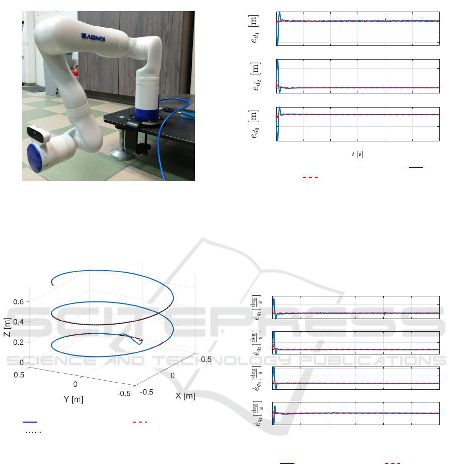
Figure 5: KINOVA

manipulator in the initial conﬁguration.

from some mechanical issues independent from the

control algorithm performance. The disturbance was

quickly compensated by the control system in both

cases and the manipulator successfully followed the

desired path.

Figure 6: Path performed by the manipulator (blue

solid Experiment, red dashed Simulation, black

dotted Desired).

In Fig. 7 path following errors are shown. In-

deed, they reveal the greater deviation measured for

the physical object at the beginning of the manoeuvre.

It is noteworthy that the obtained precision of the mo-

tion is satisfactory. Although some noise oscillations

may be observed for the experimental case, the error

signals are of the order (0.1 −1)mm. It might result

from the limited precision of mechanical elements or

sensors. Nevertheless, such precision is sufﬁcient for

autonomous path following or grasping manoeuvres.

Furthermore, Figs. 8 and 9 present errors of

following velocity proﬁles in the large and small

joints (Kinova inc., 2022), respectively. It can be ob-

served that errors for the experimental case are higher

at the beginning of the manipulator movement. It re-

sults from the mentioned above disturbances. In addi-

0 5 10 15 20 25 30

-0.04

-0.02

0 5 10 15 20 25 30

0.01

0.02

0 5 10 15 20 25 30

-0.04

-0.02

Figure 7: Path following erros e

(blue solid Experi-

ment, red dashed Simulation).

tion, the transient state lasts longer. Nonetheless, after

a short period of time there are no signiﬁcant differ-

ences between simulation and experimental results.

Moreover, all velocity proﬁle following errors tend

towards the bounds resulting from the chosen control

parameters. After a certain time the values are kept

within the bounds. Hence, the end-effector correctly

follows positions deﬁned by the helix equation (19).

0 5 10 15 20 25 30

100

200

0 5 10 15 20 25 30

100

200

0 5 10 15 20 25 30

100

0 5 10 15 20 25 30

t [s]

-50

Figure 8: Velocity proﬁle following erros ˙e

for large joints

(blue solid Experiment, red dashed Simulation).

Finally, Figs. 10 and 11 present control torques

generated for the large and small joints, respectively.

In the transient state the values generated for the

physical manipulator are higher, although the signal

changes are not as rapid as for the simulation case.

In addition, some subtle differences may be observed

during the whole manoeuvre in every joint, especially

in the ﬁrst one. It may result from the fact that in

the simulation case some factors were neglected, e.g.

friction forces. They appeared, though, in the exper-

imental case. However, despite the simpliﬁed model

in the simulation case, the obtained results do not dif-

fer signiﬁcantly and the trend of the measurements is

maintained.

Experimental Validation of the Non-Orthogonal Serret-Frenet Parametrization Applied to the Path Following Task

613

0 5 10 15 20 25 30

-60

-40

-20

0 5 10 15 20 25 30

100

0 5 10 15 20 25 30

t [s]

Figure 9: Velocity proﬁle following erros ˙e

for small joints

(blue solid Experiment, red dashed Simulation).

0 5 10 15 20 25 30

-30

-20

-10

0 5 10 15 20 25 30

-50

0 5 10 15 20 25 30

-20

-10

0 5 10 15 20 25 30

t [s]

-10

Figure 10: Control torques u for large joints (blue solid

Experiment, red dashed Simulation).

0 5 10 15 20 25 30

-20

-10

0 5 10 15 20 25 30

t [s]

-1

-0.5

Figure 11: Control torques u for small joints (blue

solid Experiment, red dashed Simulation).

All in all, the obtained experimental measure-

ments correspond with the simulation results. In spite

of the minor differences resulting from some mechan-

ical or implementation issues which arose on the lab-

oratory test–bed, the path was tracked correctly by

the real KINOVA

manipulator. Hence, it can be con-

cluded that the presented path following algorithm is

suitable for practical applications.

6 CONCLUSIONS

In the paper the path following algorithm has been

presented. It is based on two main aspects:

• the non-orthogonal Serret–Frenet parametrization

used for deriving the robot equations with respect

to the desired path (equations have the form of

a non-holonomic constraint);

• the backstepping integrator algorithm used for the

design of the control law.

The considered description is valid globally in ev-

ery point of a feasible path. Satisfying the equa-

tions resulting from the Serret–Frenet parametrization

guarantees correct path following. However, it can be

performed only via the manipulator dynamics.

As a consequence, the control system has a cas-

caded structure and the backstepping algorithm is

used to design two stages of the control cascade. The

proposed dynamic control law (the λ-tracking algo-

rithm) did not require any knowledge of the dynam-

ics parameters. However, the adaptively tuned control

gain guaranteed that the error converge to the prede-

ﬁned region. This property allowed the robot to suc-

cessfully follow the path.

The presented algorithm has been validated with

the simulation and experimental studies. The simu-

lation results were more precise. In the experiment

a disturbance at the beginning of the manoeuvre and

some noise in the measurements were observed. The

differences may result from some mechanical issues,

delays in the transmission between the computer and

the manipulator on the experimental test–bed, or sim-

pliﬁcations of the simulation model. Nonetheless, the

discrepancies were not crucial for the successful com-

pletion of the control task — the desired path was fol-

lowed correctly. The gathered experimental measure-

ments conﬁrmed that the designed algorithm can be

successfully applied to practical problems.

The results of the experiments indicate further re-

search directions. Firstly, the motion precision may

be improved. Although the achieved accuracy is sat-

isfactory for autonomous path following or even some

grasping manoeuvres, it might not be sufﬁcient for

some operations such as milling. Thus, identiﬁcation

of the dynamic structure of the manipulator may be

conducted in order to use a controller based on the

fully-known robot dynamics, or to consider some ne-

glected effects such as friction forces.

Secondly, it may be observed that the end-effector

ICINCO 2023 - 20th International Conference on Informatics in Control, Automation and Robotics

614

orientation with respect to the Serret–Frenet frame

changes during the manoeuvre. Such a behaviour may

be unfavourable in grasping processes. Hence, not

only the position control, but also the orientation con-

trol should be taken into consideration.

Finally, the control constraints could be taken into

account in the control law. It will be especially impor-

tant if the end-effector is outside the path in the initial

state. It may prevent the control system from rapid

reactions in the transient state.

REFERENCES

Cholewi

nski, M. and Mazur, A. (2019). Path tracking by

the nonholonomic mobile manipulator. In 2019 12th

International Workshop on Robot Motion and Control

(RoMoCo), pages 203–208, Poznan, Poland.

Domski, W. and Mazur, A. (2018). Path tracking with or-

thogonal parametrization for a satellite with partial

state information. In Proceedings of the 15th Interna-

tional Conference on Informatics in Control, Automa-

tion and Robotics, volume 2, pages 252–257, Porto,

Portugal.

Dyba, F. and Mazur, A. (2023). Comparison of curviline-

ar parametrization methods and avoidance of orthogo-

nal singularities in the path following task. Journal of

Automation, Mobile Robotics and Intelligent Systems.

(In press).

Encarnac¸

ao, P. and Pascoal, A. (2000). 3D path following

for autonomous underwater vehicle. In Proceedings of

the 39th IEEE Conference on Decision and Control,

pages 2977–2982, Sydney, NSW, Australia.

Hung, N., Rego, F., Quintas, J., Cruz, J., Jacinto, M.,

Souto, D., Potes, A., Sebastiao, L., and Pascoal, A.

(2023). A review of path following control strate-

gies for autonomous robotic vehicles: Theory, sim-

ulations, and experiments. Journal of Field Robotics,

40(3):747–779.

Kinova inc. (2022). Kinova Gen3 Ultra lightweight robot

user guide r8. Technical Report EN-UG-014-r8-

202210, Quebeck, Canada.

Krsti

c, M., Kanellakopoulos, I., and Kokotovi

c, P. V.

(1995). Nonlinear and Adaptive Control Design. John

Wiley & Sons, Inc., New York, USA.

Liao, Y.-L., Zhang, M.-J., and Wan, L. (2015). Serret–

Frenet frame based on path following control for un-

deractuated unmanned surface vehicles with dynamic

uncertainties. Journal of Central South University,

22:214–223.

Lugo-C

ardenas, I., Salazar, S., and Lozano, R. (2017).

Lyapunov Based 3D Path Following Kinematic Con-

troller for a Fixed Wing UAV. IFAC-PapersOnLine,

50(1):15946–15951. 20th IFAC World Congress.

Mazur, A. and Cholewi

nski, M. (2016). Implementation of

factitious force method for control of 5R manipulator

with skid-steering platform REX. Bulletin of the Pol-

ish Academy of Sciences Technical Sciences, 64(No.

1):71–80.

Mazur, A. and Dyba, F. (2023). The Non-orthogonal Serret–

Frenet Parametrization Applied to the Path Following

Problem of a Manipulator with Partially Known Dy-

namics. Archives of Control Sciences, 33(2):339–370.

Mazur, A. and Płaskonka, J. (2012). The Serret–Frenet

parametrization in a control of a mobile manipula-

tor of (nh, h) type. IFAC Proceedings Volumes,

45(22):405–410. 10th IFAC Symposium on Robot

Control.

Mazur, A., Płaskonka, J., and Kaczmarek, M. (2015). Fol-

lowing 3D paths by a manipulator. Archives of Control

Sciences, 25(1):117–133.

Mazur, A. and Schmid, C. (2000). Adaptive λ-tracking for

rigid manipulators. In Morecki, A., Bianchi, G., and

Rzymkowski, C., editors, Romansy 13. Theory and

practice of robots and manipulators., pages 103–112,

Vienna. Springer Vienna.

Mazur, A. and Szakiel, D. (2009). On path following con-

trol of nonholonomic mobile manipulators. Interna-

tional Journal of Applied Mathematics and Computer

Science, 19(4):561–574.

Micaelli, A. and Samson, C. (1993). Trajectory tracking for

unicycle-type and two-steering-wheels mobile robots.

In Technical Report No. 2097, Sophia-Antipolis.

Michałek, M. M. and Gawron, T. (2018). VFO path follow-

ing control with guarantees of positionally constrained

transients for unicycle-like robots with constrained

control input. Journal of Intelligent and Robotic Sys-

tems: Theory and Applications, 89(1-2):191 – 210.

Morro, A., Sgorbissa, A., and Zaccaria, R. (2011). Path fol-

lowing for unicycle robots with an arbitrary path cur-

vature. IEEE Transactions on Robotics, 27(5):1016–

1023.

Oprea, J. (2007). Differential Geometry and Its Appli-

cations. Prentice Hall, Washington, Cleveland State

University.

Płaskonka, J. (2013). Different kinematic path following

controllers for a wheeled mobile robot of (2,0) type.

Journal of Intelligent & Robotic Systems, 77:481–498.

Qu, Z. and Dorsey, J. (1991). Robust tracking control of

robots by a linear feedback law. IEEE Transactions

on Automatic Control, 36(9):1081–1084.

Rokonuzzaman, M., Mohajer, N., Nahavandi, S., and Mo-

hamed, S. (2021). Review and performance evaluation

of path tracking controllers of autonomous vehicles.

IET Intelligent Transport Systems, 15(5):646–670.

Selig, J. M. (2005). Geometric Fundamentals of Robotics.

Springer New York, NY, 2

edition.

Siciliano, B. and Khatib, O. (2007). Handbook of Robotics.

Springer-Verlag, Berlin, Heidelberg.

Spong, M. and Vidyasagar, M. (1991). Robot Dynamics and

Control. John Wiley & Sons, Inc., New York.

Experimental Validation of the Non-Orthogonal Serret-Frenet Parametrization Applied to the Path Following Task

615