Probabilistic Physics-Augmented Neural Networks for Robust Control

Applied to a Slider-Crank System

Edward Kikken

, Jeroen Willems

, Rob Salaets

and Erik Hostens

Flanders Make, Lommel, Belgium

ﬂ

Keywords:

Neural Networks, Physics-Augmented Neural Networks, Probablistic Neural Networks, Optimal Control,

Robust Control, Physics-Informed AI, Non-Linear Dynamic Systems Modelling.

Abstract:

Key industrial trends such as increasing energy and performance requirements as well as mass customization,

lead to more complex non-linear machines with many variants. For such systems, variability in dynamics arising

from many factors signiﬁcantly affects performance. To capture this adequately we introduce a probabilistic

extension of a Physics-Augmented Neural Network (PANN). We subsequently illustrate the added value of

such models in robust optimal control, thereby keeping performance high while guaranteeing to meet the

application’s constraints. The approach is validated on a experimental slider-crank mechanism, which is

ubiquitous in industrial machines.

1 INTRODUCTION

The industrial need for reduced energy consumption,

increased throughput and increased production ac-

curacy leads to ever-increasing performance require-

ments for mechatronic systems. These requirements

result in more complex machines with e.g., input sat-

urations, ﬂexible behavior, highly non-linear compo-

nents, many degrees of freedom (DOFs) needing to

be coordinated efﬁciently. To further complicate mat-

ters, the current trend towards mass customization

increases the number of system variants. On top of

that, intrinsic ﬂuctuations in system behavior due to

e.g., changing operating temperatures, wear, friction

lead to additional variability.

This increase in system complexity and variability

poses challenges to model and control these systems:

(i) the complex dynamics need to be accurately mod-

elled to enable high-performance control; (ii) many

models and controllers need to be developed for all

the system variants; (iii) models need to capture the

intrinsic variability; and (iv) controllers need to be sta-

ble and performant not only for the nominal dynamics,

but for the full range of variability, without resulting

in unnecessary conservative and sub-optimal control.

https://orcid.org/0000-0002-5769-5814

https://orcid.org/0000-0002-2727-6096

https://orcid.org/0000-0002-4835-0793

https://orcid.org/0000-0003-2482-7523

In industry, models targeted for model-based op-

timal control are derived from physical knowledge.

However, with ever-increasing system complexity and

variability this is becoming more-and-more labor in-

tensive and requires more-and-more expert knowledge.

The alternative approach is to build data-driven mod-

els. The methods for classical system identiﬁcation

have been around for a long time (Ljung, 1998) and

are usually employed for linear or linearized systems.

These methods have also been extended for nonlin-

ear system identiﬁcation with great effect, but often

require specialized numerical procedures (Schoukens

and Ljung, 2019). The success of Machine Learning

(ML) techniques as generic non-linear modelling tools

has motivated to use algorithms such as neural net-

works (NNs) in a Nonlinear Finite Impulse Response

(NFIR) setup or recurrent neural networks (RNNs).

They can be used to ﬁt dynamic systems using limited

expert knowledge (Forgione and Piga., 2020; Chen

et al., 2019; De Groote et al., 2021a; Beintema et al.,

2021). Furthermore, auto-differentiation as supported

by frameworks such as Pytorch (Paszke et al., 2019)

and Tensorﬂow (Abadi et al., 2015) has enabled signiﬁ-

cant computational speed-up of nonlinear system iden-

tiﬁcation. However, purely data-driven approaches

have some downsides compared to physical modelling:

they require more data since they have more parame-

ters, they extrapolate poorly outside of the operating

domain covered by the training data, and interpretabil-

ity of parameters is lost.

152

Kikken, E., Willems, J., Salaets, R. and Hostens, E.

Probabilistic Physics-Augmented Neural Networks for Robust Control Applied to a Slider-Crank System.

DOI: 10.5220/0012168200003543

In Proceedings of the 20th International Conference on Informatics in Control, Automation and Robotics (ICINCO 2023) - Volume 1, pages 152-161

ISBN: 978-989-758-670-5; ISSN: 2184-2809

To ﬁnd a middle ground between these two ap-

proaches, various approaches have been researched.

They can be organized into two main categories (Kar-

niadakis et al., 2021):

•

Physics-Inspired Neural Networks (PINNs) start

from a neural network and enforce physical laws

in the loss function of the NN (Yang et al., 2021;

Raissi et al., 2019; Schiassi et al., 2021);

•

Physics-Augmented Neural Networks (PANNs)

start with a physical model, and augment it with

NNs in its dynamic equations (De Groote et al.,

2021a; De Groote et al., 2021b).

In this work we will extend PANNs by not only mod-

elling the nominal deterministic behavior of a dynamic

system, but also its variability and uncertainty. To do

so, we will use the concept of a Probabilistic Neural

Net (PNN) (Streit and Luginbuhl, 1994; Bishop, 1994;

Lakshminarayanan et al., 2017). Modeling probability

distributions with NNs is common practice, and its

pitfalls are well known (Seitzer et al., 2022; Bishop,

1994). PNNs do not only capture aleatoric uncertainty

on the predicted outputs, but also cover the model bias

if present. Strongly linked with uncertainty modelling

are methods that estimate the epistemic uncertainty,

as represented by the parameter uncertainty, such as

Bayesian Neural Networks (Goan and Fookes, 2020),

Monte-Carlo Dropout (Gal and Ghahramani, 2016)

or Gaussian Stochastic Weight Averaging (Morimoto

et al., 2022). These works complement the techniques

in this paper, but we leave epistemic uncertainty out

of this analysis. We assume here that sufﬁcient data is

available such that the epistemic uncertainty is negligi-

ble as compared to the aleatoric uncertainty.

To control complex non-linear systems one must

move away from classical control approaches (e.g.,

PID, simple model-based or ad hoc engineered

feedforward) towards more powerful model-based

optimization-based techniques. Such methods can deal

with constraints, use preview, handle complex and non-

linear behavior and coordinate multiple DOFs (Forbes

et al., 2015), by exploiting the prediction capabilities

of dynamic models such as PANNs, see for example

(Salzmann et al., 2022; Spielberg et al., 2022; Kikken

et al., 2022). We have extended these approaches

to also include uncertainty, resulting in a robust con-

troller, inspired by the robust optimal control prob-

lem (OCP) for physical models developed in (Willems

et al., 2018).

To experimentally validate the approach, it has

been applied to a slider-crank setup that converts the

rotary movement of a motor into a linear movement.

Such mechanisms are ubiquitous in industry, e.g.,

weaving looms, piston compressors, etc. We will as-

sume some initial physical relations of the setup are

known (e.g., kinematics, some physical parameters),

but all missing dynamics will be automatically found

using the PPANN techniques.

The remainder of this paper is organized as fol-

lows. Section 2 introduces the proposed methodology.

We discuss the structure of a physics-augmented neu-

ral network and extend it to our probabilistic variant.

Next, we detail the formulation of the optimal control

problem and how it is extended to exploit the PPANN’s

uncertainty to ﬁnd a robust solution. Section 3 intro-

duces the slider-crank setup on which the developed

algorithms are experimentally validated. We explain

how we generated a dataset on this setup, on which we

have trained the PPANN that is subsequently used to

solve the robust optimal control problem. This OCP

solution is experimentally validated thereby demon-

strating the advantage of the proposed approach. Fi-

nally, we formulate our conclusions and future work

in Section 4.

2 METHODOLOGY

2.1 Notation

We consider a (non-)linear dynamic model in the form

of a set of ordinary differential equations (ODE) repre-

sented in state-space, i.e., explicit format (see Eq. 1a),

or implicit format (see Eq. 1b). These continuous-time

models are given in the form of:

˙x(t) = f (x(t), u(t), p), (1a)

0 = f (x(t), u(t), p), (1b)

where

x ∈ R

and

ˆx ∈ R

denote the measured and

(when applicable) model-predicted state variables re-

spectively (different for the two ODE variants),

u ∈

the inputs,

p ∈ R

the model parameters and func-

tion

denotes the ODE function. For the considered

class of models, we assume all states are observable,

so an output function is omitted.

When sampling time

, we denote a speciﬁc time

instant as

with

k ∈

, N

], with

the number of time

samples. For notational compactness we will denote

any time dependent signal

(

), sampled at time instant

k, as y

(and similar for e.g., u

, x

, ˙x

2.2 Combining Data-Driven and

Physical Modelling

In this section, we will ﬁrst describe the architecture of

the combined physical equations and neural networks

(PANN) and the used approach for training. Secondly,

we will extend the PANN towards the proposed proba-

bilistic modelling and training approach (PPANN).

Probabilistic Physics-Augmented Neural Networks for Robust Control Applied to a Slider-Crank System

153

2.2.1 Physics-Augmented Neural Networks

A PANN integrates a (or multiple) neural network(s)

into physical equations. These physical equations

are expressed as an explicit ODE based on lumped

physical parameters p

phys

. A PANN’s function f con-

tains the physical equations but also a neural network

that captures unmodelled phenomena

that depend on

states and/or control inputs e.g., a state dependent load,

complex friction or efﬁciency maps. For these effects

no analytical expression has been derived and they

cannot be experimentally measured directly. Note that

the inputs to the neural network are often normalized,

scaled or passed through some engineered static func-

tion, which we will denote with

. The above results

in the following general dynamic equation that is con-

sidered throughout this paper where neural network

parameters (i.e., weights and biases)

and physical

parameters p

phys

need to be identiﬁed:

˙x(t) = f (x(t), u(t), z(g(x(t), u(t)), p

), p

phys

). (2)

For notational convenience we will often write Eq. 2

in the simpliﬁed and time-sampled form:

˙x

= f (x

, u

, z

, p), (3)

where

denotes the combination of

and

phys

The derivative function of the PANN can then be prop-

agated forward in time using Euler’s method to get the

state propagation in discrete-time:

ˆx

k+1

= f (x

, u

, z

, p)∆t + x

, (4)

where ∆

denotes the time step of the forward Euler

time integration and

ˆx

k+1

the model-predicted new

state. Other time-integration schemes can also be used

of course. The PANN is graphically depicted in Fig. 1.

Figure 1: The explicit PANN model structure with time

integrator.

To ﬁt the model to the measurement data we mini-

mize the error between the model-predicted state

ˆx

and

the measured state x:

minimize

∑

k=1

− ˆx

)

(5)

The advantage of training an explicit ODE (or PANN)

using time-integration is that, when states are predicted

forward in time multiple steps, so-called N-step ahead

prediction (De Groote et al., 2021a), the optimization

becomes less sensitive to measurement noise.

Another way of formulating the dynamics of the

PANN is the implicit ODE format: a function such as

a force or torque balance that should equal zero:

0 = f (x

, u

, z

, p). (6)

When the measured states

and control inputs

are

entered into this function, the parameters

can be

optimized to minimize its left hand side, i.e., residual

at each time step k:

minimize

∑

k=1

. (7)

Note that this way of ﬁtting the model does not

require a time-integrator. However, it is more sensi-

tive to noise than N-step ahead prediction ﬁtting, also

because the measurement

needs to contain higher

derivatives (e.g., acceleration), which are harder to

measure (or estimate from measurements) accurately

and will typically exhibit greater noise levels.

2.2.2 Probabilistic Physics-Augmented Neural

Networks

In this section we will integrate the concepts of a PNN

and a PANN to ﬁnd the novel probabilistic physics-

augmented neural network (PPANN).

A PNN is a neural network architecture that re-

places a deterministic mapping of its input

(

x, u

) to

output

with a parameterized probability distribution

. In our case we choose a normal distribution

which means that the PNN outputs are the mean

and

standard deviation z

, see Fig. 2.

Figure 2: The PNN neural network architecture.

We want to train a PNN that matches the mea-

sured data and its variability as accurately as possible.

This means we want to maximize the likelihood of the

model predictions explaining the observed data. This

can be achieved using a negative log likelihood (NLL)

(Lakshminarayanan et al., 2017) cost function to train

the parameters

in the PNN. We assume that the

observed variability can be captured in a Gaussian

(i.e., normal) distribution, so we can use the following

expression for the NLL cost:

minimize

∑

k=1



− z

)

σ2

+ log((z

)



, (8)

ICINCO 2023 - 20th International Conference on Informatics in Control, Automation and Robotics

154

where

denotes the measured output that is captured

by the PNN.

Interconnecting the PNN and the PANN is rather

straightforward and depicted in Fig. 3. However, we

Figure 3: The implicit PPANN model structure.

want to predict

and

using the data we measure

on the complete system: we do not have a direct mea-

surement

. To resolve this, we must propagate

and

of the neural network to the PPANN residual

output

, which results in the following modiﬁed NLL

optimization to train PPANN’s:

minimize

∑

k=1





(

)

+ log(

)





. (9)

This cost function can easily be extended when multi-

ple PNN are inserted into the PANN.

There are however two drawbacks related to train-

ing the PPANN using the cost described in Eq. 9. The

ﬁrst is related to our earlier remark that with the im-

plicit formulation we cannot use the N-step ahead pre-

diction for training. Secondly, there is a risk that the

optimization gets stuck in a local optimum where the

mean model

ﬁts poorly which is compensated with a

large

to explain the measured data. Yet, although we

can easily propagate

N steps ahead in time through

the explicit ODE, the same cannot be done as straight-

forwardly for

. Therefore, to ensure we get an accu-

rate mean prediction and limit the model bias, but in

the same time still allow for the probabilistic extension,

we split the training approach in two phases:

Train the mean neural network

of the PPANN

using N-step ahead prediction with a MSE cost

function. Note that the MSE cost is equivalent to

assuming

is constant, therefore

will not run

away to compensate for a poor z

ﬁt.

Fix

and train the sigma network

of the

PPANN using the NLL cost from Eq. 9.

2.3 Optimal Control

The formulation of a generic discrete-time optimal

control problem is:

minimize

x,u

OCP

(x, u) (10a)

s. t. x

k+1

= f (x

, u

, z

, p)∆t + x

, ∀ k ∈ [1, N]

(10b)

h ≤ h(x, u) ≤

h. (10c)

In the above, Eq. 10a denotes the cost function which

can depend on states and/or inputs, Eq. 10b imple-

ments the model dynamics using a multiple shooting

approach, see (Bock and Plitt, 1984) for more details.

Finally, Eq. 10c implements the desired constraints

(e.g., initial condition, input and path constraints)

lower and upper bounded by h and

The resulting discrete-time optimization problem

is a large-but-sparse non-linear program (NLP), con-

taining continuous optimization variables. We will

use the CasADi framework (Andersson et al., 2019)

to efﬁciently set-up the problem, which employs algo-

rithmic differentiation, and we will solve it using the

gradient-based interior point optimization algorithm

IPOPT (Wächter and Biegler, 2006).

2.4 Robust Optimal Control Using

Probabilistic Physics-Augmented

Neural Networks

In this section, we will describe the extension of the

optimal control problem of Section 2.3 to a robust

OCP leveraging the dynamics captured in the PPANN.

As shown in the previous section, we can embed

state-space model dynamics, for example of a PANN

or PPANN, in the optimization problem. Ideally one

would also add the PPANN’s description of uncertainty

to the OCP to formulate constraints with respect to

the uncertain dynamics. However, since there is no

explicit formulation for the propagation of uncertainty

in time this can not be done. Instead, we will compute

the uncertainty in time by, at each time step

, Monte

Carlo sampling

times the distribution ﬁtted by the

PPANN to get

( j)

and performing the time integration

of the dynamics for each k and j as:

ˆx

( j)

k+1

= f (x

, u

, z

( j)

, p)∆t + x

, (11)

If we stack these varying state propagations into

ˆx

, we can once again compute a standard deviation

(

ˆx

). This can then be used to compute the 3

upper and lower bound of the states. These bounds

can be used to add a robustness safety margin to the

state constraint (Eq. 10c) after which the OCP can be

solved again with the updated constraints.

Probabilistic Physics-Augmented Neural Networks for Robust Control Applied to a Slider-Crank System

155

3 EXPERIMENTAL RESULTS

In this section, we explain the approach proposed in

Section 2 applied to a lab-scale slider-crank mecha-

nism designed to mimic weaving looms and similar

industrial systems. First, we introduce the setup and

generate a dataset. Secondly, we train the PPANN on

the dataset and lastly, we solve a robust optimal control

problem and validate its performance on the setup.

3.1 Slider-Crank Mechanism

We consider the control of a slider-crank mechanism,

which is shown schematically in Fig. 4. The mech-

anism converts a rotary motion

θ ∈ R

into a linear

displacement

slider

∈ R

using input torque

τ ∈ R

- a

motion conversion that often emerges in industrial ap-

plications, such as weaving looms, compressors and

piston engines. The system contains non-linearities

and has dead points. The state vector of the system is

deﬁned as



θ ω



, with angular velocity

and input u = τ.

The slider displacement

slider

is calculated using

a straightforward kinematic function that is assumed

to be known:

slider

cos

(

) +

cos

(

) +

− l

employing geometric constraint

sin

−1

(

sin

(

)).

The crank-arm length

= 0.05 m and connecting-rod

length is set to

= 0.3 m respectively. Furthermore,

we have approximate values for inertia (

= 3

−3

kg/m

), damping (

= 0.1 Ns/rad) and the stiffness

= 1 N/rad).

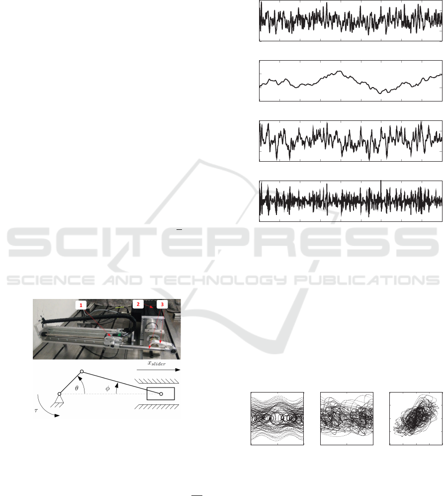
Figure 4: Picture and schematic overview of the slider-crank

system consisting of: (1) linear slider, (2) rotary motor and

(3) the crank and connecting rod.

3.2 Dataset Generation

We sample the measurements at 500 Hz (∆

500

and generate 90 seconds of data. In order to excite

the system, we have generated a semi-random input

torque (which is ﬁltered by a low-pass ﬁlter), as shown

in the top plot of Fig. 5. Furthermore, to increase

the variability of the system and better validate our

method, we have applied a white-noise input force on

the slider with a peak amplitude of 30 N (which acts as

a non-measured disturbance). Applying these inputs

results in the measured state evolution as shown in

Fig. 5.

0 10 20 30 40

50 60

70 80 90

−10

−5

Time [s]

Torque [Nm]

0 10 20 30 40

50 60

70 80 90

−50

100

Time [s]

Angle [rad]

0 10 20 30 40

50 60

70 80 90

−100

−50

100

Time [s]

Angular velocity [rad/s]

0 10 20 30 40

50 60

70 80 90

−2,500

2,500

Time [s]

Angular acc. [rad/s

]

Figure 5: The input torque considered to excite the physical

system and the measured states of the physical model after

excitation with the given input torque.

In Fig. 6, the coverage maps are shown for the

entire dataset. It can be seen that the maps are quite

densely populated, i.e., the training data is quite rich

(within the considered bounds that are chosen large

enough to ensure that the OCP solution falls within

them), which is required for an accurate ﬁt of the

PPANN. Note that the angles are plotted between 0

and 2

, since it is assumed that the system is periodic

over each rotation.

2π

−100

−50

100

Angle [rad]

Velocity [rad/s]

2π

−10

−5

Angle [rad]

Torque [Nm]

−100

−50

100

−10

−5

Velocity [rad/s]

Torque [Nm]

Figure 6: The coverage maps of the dataset.

3.3 PPANN Design and Training

In this section, we will discuss the architecture of the

PPANN model for the considered slider-crank system

and then execute the training, using the dataset created

in the previous section.

ICINCO 2023 - 20th International Conference on Informatics in Control, Automation and Robotics

156

3.3.1 Parameterization of the Considered

PPANN

The state propagation function of the considered

PPANN (explicit form) is given as follows:

˙x

= f (x

, u

, z

, p) =



α(x

, u

, z

, p)



. (12)

We exploit the fact that for the given system,

, i.e.,

the derivative of the ﬁrst state is equal to the second

state. Therefore, it is not needed to have the PPANN

predict both states, we will instead let it predict the

derivative of the second state, i.e.,

. As a result,

the relation between

and

remains maintained even

in case of an imperfect model.

In the above, function

denotes the mapping from

state and input to the inputs of the PPANN. Instead

of using the states of the slider crank system (and

its input) directly as input, i.e.,



θ ω τ



∈ R

we use:

(

x, u

) =



sin(θ) cos(θ) ω τ



∈ R

thereby constraining the input space of the neural net-

works. It is equivalent to imposing a 2

periodicity

over the angle θ.

In order to derive function

, we ﬁrst employ a

simple and generic 2

order linear system:

lin

, u

, p

phys

) =

− B

− K

mod

. (13)

In the above,

phys





, and

mod

equal to

modulo 2

. Second, the above linear model

is augmented to a PPANN (yielding

from Eq. 12),

by employing three neural networks z

µJ

, z

µB

and z

µK

α(x

, u

, z

, p) =

− B

(1 + z

µB

)ω

− K

(1 + z

µK

)θ

mod

(1 + z

µJ

)

(14)

In the above, three separate neural networks are

present, the mean inertia network output

µJ

, mean

damping network

µB

and mean stiffness network

µK

which allow the additional (non-)linear dynamics to

be modelled as well. Note that networks

µJ

and

µK

are parameterized to be a function of only (the trans-

formed)

, i.e.,



sin(θ) cos(θ)



, thereby allowing

for a position-dependent inertia and stiffness proﬁle.

µB

is parameterized to be a function of both (the trans-

formed)

and

, i.e.,



sin(θ) cos(θ) ω



, allow-

ing not only position dependency to be accounted for,

but also speed-dependent effects (e.g., Stribeck fric-

tion).

For the

networks of the PPANN, each is con-

structed using a single hidden layer of 100 neurons,

which is shown to be able to to approximate any con-

tinuous function (Hornik et al., 1989). We have used a

linear activation function for the ﬁnal layer (the output

layer), and

tanh

activations for the previous layers. For

the z

networks, each of the three uses 10 neurons.

3.3.2 Training the PPANN

Now that the architecture has been deﬁned, we will use

the dataset obtained in Section 3.2 to train the neural

networks. We use the ﬁrst 87 seconds for training, and

the last 3 seconds for validation. A learning rate of

−3

is used for the Adam optimizer (Kingma and Ba,

2014). As described in Section 2.2.2, we ﬁrst train the

part of the PPANN (using cost function given by Eq.

5 and N-step ahead training with a prediction horizon

= 10) and afterwards, the

part of the PPANN

is trained (employing Eq. 9).

The resulting 3-D maps for each of the six net-

works trained are shown in Fig. 7. We make the fol-

lowing observations:

•

For the inertia maps (top row), oscillatory behavior

can be seen for the

µJ

network: the inertia varies

as a function of the angle, due to the kinematic rela-

tion between motor rotation and slider translation.

When the crank and connecting rod are parallel

to each other (

{

, π,

π}

), the perceived in-

ertia is the lowest (dead points), and highest at

(

{

π,

π}

). The uncertainty is the highest

when the crank and rocker are in the upper posi-

tion (between 0 and

), but compared to the other

networks it is small.

•

For the damping maps (middle row), again and

varying behavior can be seen as a function of angle

and velocity. The damping seems to be the highest

around low speeds, when the crank and rod are

approximately perpendicular (e.g., due to stick-slip

friction present on the slider), and again increases

for higher speeds (viscous friction in the rotary

motor).

•

For the spring maps (bottom row), it can be seen

that the

network oscillates around -1. Since this

thus almost cancels out the stiffness related term

(

(1 +

µK

)

mod

), in Eq. 14, the contribution of

stiffness to the total torque is thus rather limited.

The remaining part can for example be attributed to

effects such as cogging and ﬂexibility of the setup.

The uncertainty is the highest when the crank and

rocker are in the upper position (between 0 and

In Fig. 8, the output of the

part of the trained

PPANN (deterministic part) is shown for the entire

validation dataset. It can be seen that a good match is

obtained between the validation data and the prediction

of the neural network, even for longer prediction hori-

zons (in this case: 3 seconds). The observed mismatch

can be attributed to variability in the behavior, such as

(non-measured) white noise force excited by the linear

Probabilistic Physics-Augmented Neural Networks for Robust Control Applied to a Slider-Crank System

157

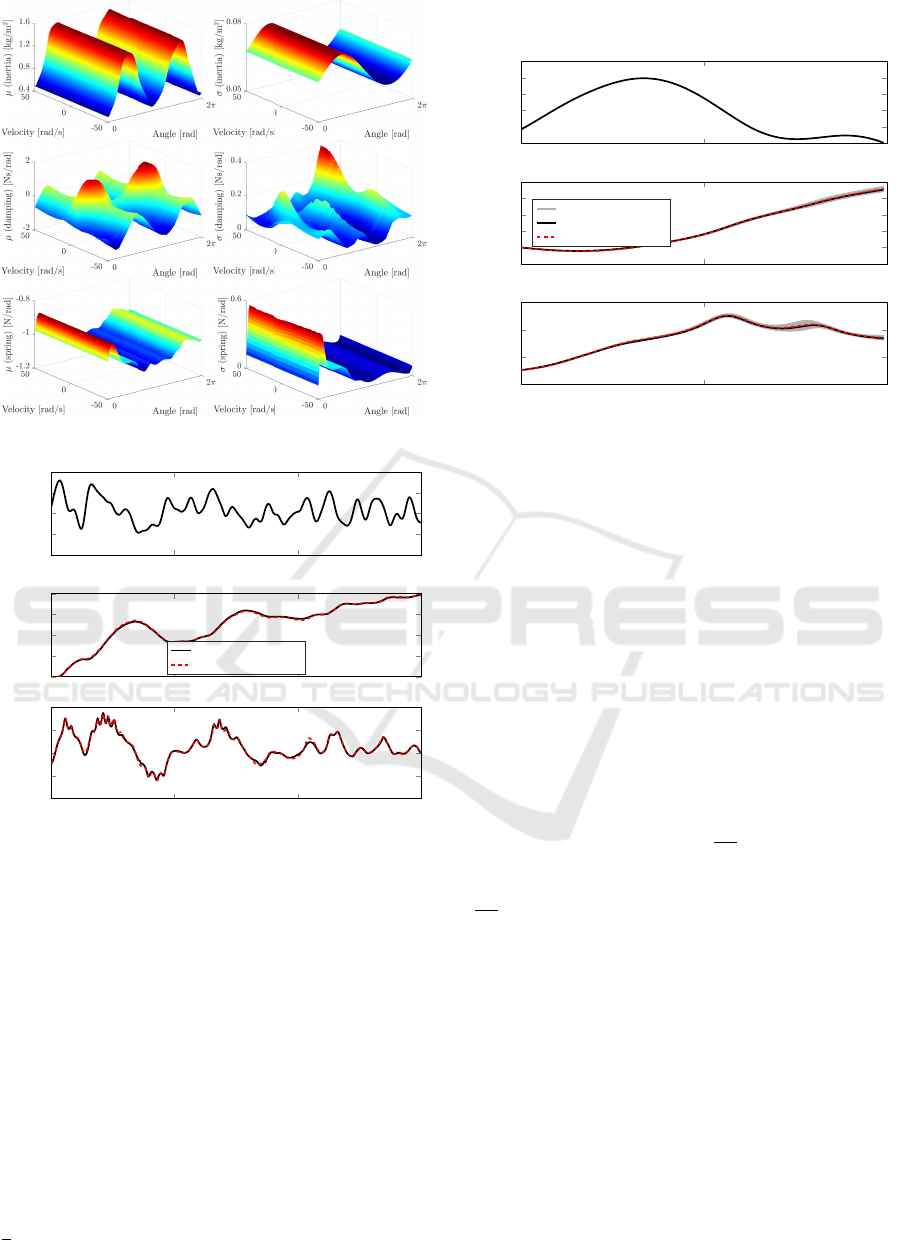
Figure 7: Resulting 3-D maps for the µ and σ networks.

0 1 2 3

−10

−5

Time [s]

Torque [Nm]

0 1 2 3

Time [s]

Angle [rad]

Validation data

Forward simulation (µ)

0 1 2 3

−100

−50

100

Time [s]

Angular velocity [rad/s]

Figure 8: The results of the trained PPANN demonstrated on

the validation dataset.

motor acting on the slider, as well as backlash in the

setup.

Next, we demonstrate the uncertainty part captured

by the trained PPANN, by including the (stochastic)

nets as well in the simulation. To do so, we have

employed Monte Carlo sampling (see Eq. 11); sam-

pling the trained model 100 times (yielding

ˆx

( j)

with

= 1

, . . . ,

100). In this way we obtain a varying state

propagation, on which we can compute the standard

deviation at each time step, similar to as discussed in

Section 2.4, allowing to compute the 3

upper and

lower bounds. The results are shown in Fig. 9. We

have shown the original validation data and forward

simulation of the deterministic part (

), as well as the

and

¯x

bounds: forming a state and time-propagation

dependent uncertainty band around the deterministic

part.

0 0.1 0.2

Time [s]

Torque [Nm]

0 0.1 0.2

−2

Time [s]

Angle [rad]

3σ bounds

Validation data

Forward simulation (µ)

0 0.1 0.2

−50

100

Time [s]

Angular velocity [rad/s]

Figure 9: Uncertainty simulation on part of validation

dataset.

3.4 Optimal Control and Results

In this section, we will solve a typical control case for

such an oscillating mechanism using the robust OCP

approach described in Sections 2.3 and 2.4. We use

the trained PPANN, and validate the results by running

it multiple times on the physical setup to verify if the

solution indeed performs robustly.

3.4.1 Problem Formulation

First, we will solve an optimal control problem that

minimizes the input torque, while meeting several

constraints on the states. We set up the optimal con-

trol problem denoted in Eq. 10, with cost function

OCP

∑

k=1

+ 1

−4

∑

N−1

k=1

(

∆u

)

, where ∆ denotes

the discrete derivative operator. We set the horizon

length

to 150 samples, and use a sampling time of

500

s. Additionally, the following motion constraints

are taken into account:











slider

≥ 0.08, k ∈

{

50, 100

}

= π, ω

= 0,

= 3π, ω

= 0.

(15)

The ﬁrst constraint involves the height (0.08 m) and

timing (samples 50 and 100) of the displacement of

the slider. The second and third constraint denote the

initial and ﬁnal angular conditions.

3.4.2 Step 1: Solve non-Robust OCP (Without

Uncertainty)

Using the model trained in the previous section, we

have solved the OCP. The results are shown in Fig. 10.

ICINCO 2023 - 20th International Conference on Informatics in Control, Automation and Robotics

158

The top plot shows the calculated input torque, and the

bottom plot shows the slider displacement calculated

using the mean PPANN, as well as the given constraint

surface. It can be seen that the nominal OCP result

(calculated on the mean PPANN) satisﬁes the given

constraints.

0.15

0.3

−6

Time [s]

Torque [Nm]

0.15

0.3

0.02

0.04

0.06

0.08

0.1

Time [s]

Displacement [m]

Constraint

OCP (µ)

3σ bounds

Figure 10: OCP results (non-robust case) solved using the

mean PPANN. The 3

bounds are computed and shown

afterwards.

3.4.3

Step 2: Determine Uncertainty (Given OCP

Solution)

Next, the 3

standard deviation on the slider dis-

placement, denoted by 3

(

slider, MC

), is calculated

by Monte Carlo sampling the PPANN with variability

(using 100 trajectories, see Eq. 11). In Fig. 10, it can

be seen that if uncertainty is accounted for, satisfaction

of the constraints is not guaranteed.

3.4.4 Step 3: Solve Robust OCP (Accounting for

Uncertainty)

In this step, the goal is to solve a robust OCP, i.e., an

OCP which guarantees constraint satisfaction given

the modelled uncertainty. To do so, we update the

constraints on the slider displacement (see Eq. 15) to:

slider

− 3σ(x

slider, MC

) ≥ 0.08, k ∈

{

50, 100

}

. (16)

Note that only the lower bound

−

case is consid-

ered, since it is the only active constraint. The results

are shown in Fig. 11. The top plot shows the (previ-

ously computed) non-robust and robust input torque,

which does account for the uncertainty. The bottom

plot shows the resulting slider displacement calculated

using the robust OCP and its 3

bounds, again com-

puted using Monte Carlo simulation. In the ﬁgure, it

can be seen that the updated result is indeed feasible,

given the (re-computed) uncertainty. Note that for this

example we were able to obtain a robust solution by

solving the OCP twice (once for the nominal case and

once for the case accounting for uncertainty). Note

that multiple iterations could be considered in case

the uncertainty would change more between operating

regions.

0.15

0.3

−6

Time [s]

Torque [Nm]

Non-robust

Robust

0.15

0.3

0.02

0.04

0.06

0.08

0.1

Time [s]

Displacement [m]

Constraint

OCP (µ)

3σ bounds

Figure 11: OCP results (robust case), accounting for uncer-

tainty.

3.5 Implementation on Physical Setup

In this section, we will implement the OCP results

determined in the previous section on the physical

setup, to validate the approach presented in this paper.

We have applied both the input signals computed in

the previous section (non-robust and robust case) 100

times each. In Fig. 12 the results are shown: the con-

straint box, the slider displacement computed by the

OCP in simulation, the mean displacement measured

on the experimental setup and the corresponding 3

bounds (calculated on the experimental data). The top

plot shows the result for the non-robust case. Sim-

ilar to as shown in simulation, if uncertainty is not

accounted for, the constraints can be violated. The

bottom plot shows the robust case, where uncertainty

is accounted for. In this case, it can be seen that the

constraints are indeed satisﬁed. Note that however the

band seems to be smaller for the experimental case

compared to the simulation case (see Fig. 11). This

could be attributed to for example imperfections (bias)

in the training of the

network, or reduced heating up

of the setup (thereby changing the friction), compared

to the longer duration training data.

4 CONCLUSIONS

In this work we demonstrated an approach to augment

a physical model with probabilistic neural networks

to capture unmodelled effects. It predicts not only

the mean system behavior but also its variance. We

coined this novel model structure PPANN. Prediction

of the mean and variance was exploited using a robust

optimal control approach, where the predicted vari-

Probabilistic Physics-Augmented Neural Networks for Robust Control Applied to a Slider-Crank System

159

0.15

0.3

0.02

0.04

0.06

0.08

0.1

Time [s]

Displacement [m]

Non-robust

Constraint

OCP (exp.) (µ)

OCP (sim.) (µ)

3σ bounds (exp.)

0.15

0.3

0.02

0.04

0.06

0.08

0.1

Time [s]

Displacement [m]

Robust

Constraint

OCP (exp.) (µ)

OCP (sim.) (µ)

3σ bounds (exp.)

Figure 12: Results of the experimental validation, for both

the non-robust and robust case.

ability was included in the control optimization con-

straints to ensure the necessary robustness. Validation

of the PPANN model and the robust optimal control

approach was performed on a slider-crank setup mim-

icking an industrial weaving loom. It was shown that

the PPANN captured the mean system behavior, but

also its variability, as intended. Furthermore, the ro-

bust controller was shown to have (near-)minimal but

sufﬁcient robustness. The constraints were satisﬁed

whilst achieving high performance thereby validating

the approach on a real system.

Future work will look into the following topics:

•

Research how to meaningfully propagate uncer-

tainty in time and train both model mean and vari-

ance using N-step ahead predictions. This will

also allow us to directly include variability in the

robust OCP and remove the need for iterative OCP

solving.

•

Train the PPANN in a single shot, as opposed to

the current two-phase approach, whilst ﬁnding the

minimal uncertainty.

•

Research into training physical and neural parame-

ters at the same time, whilst maximizing the con-

tribution of physical parameters (which have the

advantage of extrapolation beyond the trained re-

gion).

•

Add uncertainty to the physical parameters in case

there is reason to assume these are probabilistic.

•

Applying the current (off-line) optimal control

problem in an (on-line) model-predictive control

setting.

ACKNOWLEDGMENTS

This work has been carried out within the framework

of Flanders Make’s IRVA project HAIEM (Hybrid AI

for Estimation in Mechatronics), funded by Flanders

Make and the AI Research Program of the Flemish

Government. Flanders Make is the Flemish strategic

research centre for the manufacturing industry.

REFERENCES

Abadi, M., Agarwal, A., Barham, P., Brevdo, E., Chen, Z.,

Citro, C., Corrado, G. S., Davis, A., Dean, J., Devin,

M., Ghemawat, S., Goodfellow, I., Harp, A., Irving, G.,

Isard, M., Jia, Y., Jozefowicz, R., Kaiser, L., Kudlur,

M., Levenberg, J., Mané, D., Monga, R., Moore, S.,

Murray, D., Olah, C., Schuster, M., Shlens, J., Steiner,

B., Sutskever, I., Talwar, K., Tucker, P., Vanhoucke,

V., Vasudevan, V., Viégas, F., Vinyals, O., Warden,

P., Wattenberg, M., Wicke, M., Yu, Y., and Zheng, X.

(2015). TensorFlow: Large-scale machine learning

on heterogeneous systems. Software available from

tensorﬂow.org.

Andersson, J. A. E., Gillis, J., Horn, G., Rawlings, J. B.,

and Diehl, M. (2019). CasADi – A software frame-

work for nonlinear optimization and optimal control.

Mathematical Programming Computation, 11(1):1–36.

Beintema, G., Toth, R., and Schoukens, M. (2021). Non-

linear state-space identiﬁcation using deep encoder

networks. In Learning for dynamics and control, pages

241–250. PMLR.

Bishop, C. (1994). Mixture density networks. Workingpaper,

Aston University.

Bock, H. G. and Plitt, K.-J. (1984). A multiple shooting al-

gorithm for direct solution of optimal control problems.

IFAC Proceedings Volumes, 17(2):1603–1608.

Chen, R. T. Q., Rubanova, Y., Bettencourt, J., and Duve-

naud, D. (2019). Neural ordinary differential equations.

arXiv preprint arXiv:1806.07366.

De Groote, W., Kikken, E., Hostens, E., Van Hoecke, S.,

and Crevecoeur, G. (2021a). Neural network aug-

mented physics models for systems with partially un-

known dynamics: application to slider–crank mech-

anism. IEEE/ASME Transactions on Mechatronics,

27(1):103–114.

De Groote, W., Van Hoecke, S., and Crevecoeur, G. (2021b).

Physics-based neural network models for prediction

of cam-follower dynamics beyond nominal opera-

tions. IEEE/ASME Transactions on Mechatronics,

27(4):2345–2355.

Forbes, M. G., Patwardhan, R. S., Hamadah, H., and

Gopaluni, R. B. (2015). Model predictive control

in industry: Challenges and opportunities. IFAC-

PapersOnLine, 48(8):531–538.

Forgione, M. and Piga., D. (2020). Model structures and

ﬁtting criteria for system identiﬁcation with neural

networks. 2020 IEEE 14th International Conference

ICINCO 2023 - 20th International Conference on Informatics in Control, Automation and Robotics

160

on Application of Information and Communication

Technologies (AICT), pages 1–6. IEEE, 2020.

Gal, Y. and Ghahramani, Z. (2016). Dropout as a bayesian ap-

proximation: Representing model uncertainty in deep

learning.

Goan, E. and Fookes, C. (2020). Bayesian neural networks:

An introduction and survey. In Case Studies in Ap-

plied Bayesian Data Science, pages 45–87. Springer

International Publishing.

Hornik, K., Stinchcombe, M., and White, H. (1989). Multi-

layer feedforward networks are universal approxima-

tors. Neural networks, 2(5):359–366.

Karniadakis, G., Kevrekidis, Y., Lu, L., Perdikaris, P., Wang,

S., and Yang, L. (2021). Physics-informed machine

learning. Nature Reviews Physics, 3:422–440.

Kikken, E., Depraetere, B., and Willems, J. (2022). Bridging

dynamic neural networks and optimal control. In 41st

Benelux Meeting on Systems and Control, Brussels,

Belgium.

Kingma, D. P. and Ba, J. (2014). Adam: A

method for stochastic optimization. arXiv preprint

arXiv:1412.6980.

Lakshminarayanan, B., Pritzel, A., and Blundell, C. (2017).

Simple and scalable predictive uncertainty estimation

using deep ensembles.

Ljung, L. (1998). System Identiﬁcation, pages 163–173.

Birkhäuser Boston, Boston, MA.

Morimoto, M., Fukami, K., Maulik, R., Vinuesa, R., and

Fukagata, K. (2022). Assessments of epistemic uncer-

tainty using gaussian stochastic weight averaging for

ﬂuid-ﬂow regression. Physica D: Nonlinear Phenom-

ena, 440:133454.

Paszke, A., Gross, S., Massa, F., Lerer, A., Bradbury, J.,

Chanan, G., Killeen, T., Lin, Z., Gimelshein, N.,

Antiga, L., Desmaison, A., Kopf, A., Yang, E., DeVito,

Z., Raison, M., Tejani, A., Chilamkurthy, S., Steiner,

B., Fang, L., Bai, J., and Chintala, S. (2019). Pytorch:

An imperative style, high-performance deep learning

library. In Advances in Neural Information Processing

Systems 32, pages 8024–8035. Curran Associates, Inc.

Raissi, M., Perdikaris, P., and Karniadakis, G. (2019).

Physics-informed neural networks: A deep learning

framework for solving forward and inverse problems

involving nonlinear partial differential equations. Jour-

nal of Computational Physics, 378:686–707.

Salzmann, T., Kaufmann, E., Pavone, M., Scaramuzza, D.,

and Ryll, M. (2022). Neural-mpc: Deep learning model

predictive control for quadrotors and agile robotic plat-

forms. arXiv preprint arXiv:2203.07747.

Schiassi, E., Furfaro, R., Leake, C., De Florio, M., John-

ston, H., and Mortari, D. (2021). Extreme theory of

functional connections: A fast physics-informed neu-

ral network method for solving ordinary and partial

differential equations. Neurocomputing, 457:334–356.

Schoukens, J. and Ljung, L. (2019). Nonlinear system iden-

tiﬁcation: A user-oriented road map. IEEE Control

Systems Magazine, 39(6):28–99.

Seitzer, M., Tavakoli, A., Antic, D., and Martius, G. (2022).

On the pitfalls of heteroscedastic uncertainty estima-

tion with probabilistic neural networks. arXiv preprint

arXiv:2203.09168.

Spielberg, N. A., Brown, M., and Gerdes, J. C. (2022). Neu-

ral network model predictive motion control applied to

automated driving with unknown friction. IEEE Trans-

actions on Control Systems Technology, 30(5):1934–

1945.

Streit, R. L. and Luginbuhl, T. E. (1994). Maximum likeli-

hood training of probabilistic neural networks. IEEE

Transactions on neural networks, 5(5):764–783.

Wächter, A. and Biegler, L. T. (2006). On the implemen-

tation of an interior-point ﬁlter line-search algorithm

for large-scale nonlinear programming. Mathematical

programming, 106(1):25:57.

Willems, J., Hostens, E., Depraetere, B., Steinhauser, A.,

and Swevers, J. (2018). Learning control in practice:

Novel paradigms for industrial applications. In IEEE

Conference on Control Technology and Applications

(CCTA).

Yang, L., Meng, X., and Karniadakis, G. E. (2021). B-pinns:

Bayesian physics-informed neural networks for for-

ward and inverse pde problems with noisy data. Jour-

nal of Computational Physics, 425:109913.

Probabilistic Physics-Augmented Neural Networks for Robust Control Applied to a Slider-Crank System

161