Equidistant Reorder Operator for Cartesian Genetic Programming

Henning Cui

1 a

, Andreas Margraf

2 b

and J

org H

ahner

1 c

Institute for Computer Science, University of Augsburg, Am Technologiezentrum 8, 86159 Augsburg, Germany

Fraunhofer IGCV, Am Technologiezentrum 2, 86159 Augsburg, Germany

Keywords:

Cartesian Genetic Programming, CGP, Mutation Operator, Reorder, Genetic Programming, Evolutionary

Algorithm.

Abstract:

The Reorder operator, an extension to Cartesian Genetic Programming (CGP), eliminates limitations of the

classic CGP algorithm by shufﬂing the genome. One of those limitations is the positional bias, a phenomenon

in which mostly genes at the start of the genome contribute to an output, while genes at the end rarely do.

This can lead to worse ﬁtness or more training iterations needed to ﬁnd a solution. To combat this problem,

the existing Reorder operator shufﬂes the genome without changing its phenotypical encoding. However, we

argue that Reorder may not fully eliminate the positional bias but only weaken its effects. By introducing a

novel operator we name Equidistant-Reorder, we try to fully avoid the positional bias. Instead of shufﬂing the

genome, active nodes are reordered equidistantly in the genome. Via this operator, we can show empirically

on four Boolean benchmarks that the number of iterations needed until a solution is found decreases; and

fewer nodes are needed to efﬁciently ﬁnd a solution, which potentially saves CPU time with each iteration. At

last, we visually analyse the distribution of active nodes in the genomes. A potential decrease of the negative

effects of the positional bias can be derived with our extension.

1 INTRODUCTION

Cartesian Genetic Programming (CGP) is a form

of Genetic Programming (GP), based on directed

acyclic graphs whose nodes are arranged in a two-

dimensional grid.

Since its inception in 1999 by Miller, CGP has

been used for various applications (Miller, 1999).

Originally, Miller used it to evolve digital cir-

cuits (Miller, 1999), which is still a use case to this

day (Froehlich and Drechsler, 2022; Manazir and

Raza, 2022). Furthermore, the CGP concept is used

in a diverse ﬁeld of problem domains like classiﬁca-

tion or regression (Miller, 2011). Other works uti-

lized CGP for image segmentation (Leitner et al.,

2012; Margraf et al., 2017) or the evaluation of sensor

data (Huang et al., 2022; Bentley and Lim, 2017).

CGP has some advantages over GP, such as the

absence of bloat (Miller, 1999): Solutions becom-

ing larger without an increase in ﬁtness. However,

there are also some downsides and limitations in CGP.

One of those limitations is its positional bias, an ef-

https://orcid.org/0000-0001-5483-5079

https://orcid.org/0000-0002-2144-0262

https://orcid.org/0000-0003-0107-264X

fect which potentially limits CGP to fully explore

its search space (Goldman and Punch, 2013a). To

counteract this problem, Goldman and Punch intro-

duced Reorder, an operator to shufﬂe CGPs genome

ordering without changing its phenotype (Goldman

and Punch, 2013a). However, we believe that Re-

order suffers from some limitations, too, which could

lead to the search space being explored inefﬁciently.

This, in turn, could increase the iterations needed for

training as CGP gets stuck in local optima. To miti-

gate this problem, we introduce a modiﬁcation to Re-

order: Equidistant-Reorder. With our modiﬁcation,

the genome is not shufﬂed randomly anymore. By

additionally inﬂuencing the genomes reordering, the

effects of the positional bias may be further lessened.

In turn, CGP with Equidistant-Reorder needs less it-

erations to ﬁnd a solution, which can save computa-

tional time.

In the following Section 2, we provide a quick

overview of the core principles of CGP and reintro-

duce the Reorder operator. Afterwards, Section 3

gives an overview of related work. In Section 4,

we discuss the aforementioned limitation of Reorder

more in-depth. Furthermore, we formally introduce

and explain our operator: Equidistant-Reorder. Af-

Cui, H., Margraf, A. and Hähner, J.

Equidistant Reorder Operator for Cartesian Genetic Programming.

DOI: 10.5220/0012174100003595

In Proceedings of the 15th International Joint Conference on Computational Intelligence (IJCCI 2023), pages 64-74

ISBN: 978-989-758-674-3; ISSN: 2184-3236

terwards, its performance is analysed using several

Boolean benchmark problems in Section 5. At last,

Section 6 summarizes our ﬁndings and discusses fu-

ture research directions.

2 CARTESIAN GENETIC

PROGRAMMING

In the following section, the core principles of the su-

pervised learning algorithm called Cartesian Genetic

Programming (CGP) is reintroduced. In addition, the

CGP’s extension Reorder by Goldman and Punch is

presented (Goldman and Punch, 2013a).

The standard CGP variant described in Section 2.1

will be called STANDARD in the next sections to im-

prove readability. Apart from that, a CGP variant with

the Reorder operator employed will be called RE-

ORDER.

2.1 Representation

Traditionally, CGP is represented as a directed,

acyclic and feed-forward graph. This graph contains

nodes which are arranged in a c × r grid, with c ∈ N

and r ∈ N

deﬁning the number of columns and rows

in the grid respectively. Given an arbitrary amount

of program inputs, the CGP model feeds those inputs

forward through its partially connected nodes to get

any desired amount of outputs. Please note that, with

today’s standards, a CGP model typically consists of

only one row (Miller, 2011). That means, r = 1.

The set of nodes can be divided into three groups:

input-, computational- and output-nodes. Input nodes

directly receive a program input. Their only purpose

is to relay the program input. Differently, computa-

tional nodes are represented by a function gene and

a connection genes. Here, a ∈ N

is the maximum

arity of all functions in the predeﬁned function set,

while the function gene addresses the encoded com-

putational function of the node. Please note that if a

function needs less than a inputs, all excessive input

genes are ignored. At last, output nodes redirect the

calculated output of a computational node and deﬁne

the model’s output. They are represented by a sin-

gle connection gene, which deﬁnes a path between a

previous node and the current node.

In this sense, when we mention a graph with

N ∈ N

nodes, this graph will have only one row, N

computational nodes and additional input and output

nodes corresponding to the given learning task.

Another important distinction of computational

nodes are active and inactive nodes. Active nodes are

part of a path to an output node. Hence, they actively

INPUT

ADD

SUB

ADD

OUTPUT

Figure 1: Example graph deﬁned by a CGP genotype. The

dashed node and connections are inactive due to not con-

tributing to the output.

contribute to a program output. On the contrary, inac-

tive nodes do not contain a path to an output node and

do not contribute to the model’s output. However, in-

active nodes are essential to CGP as they probably aid

the evolutionary process through genetic drift (Turner

and Miller, 2015).

An illustrative example of a graph deﬁned by a

CGP genotype can be seen in Figure 1. It shows a

graph with c = 6 and r = 1, which is supposed to solve

a task consisting of two inputs and one output. Here,

the ﬁrst two nodes (n

and n

) are input nodes and

provide two different program inputs. The follow-

ing nodes (n

–n

) are computational nodes. At last,

the output is provided by one output node n

. In this

example, both inputs are subtracted, with this inter-

mediate result being added to itself and taken as the

program output. Thus, every node drawn with a solid

line is an active node. The node n

is an inactive node

(marked by dashed lines) since it does not contribute

to the program output nor contains a path to an output

node.

2.2 Evolutionary Algorithm Used by

CGP

As is standard in most CGP variants, an elitist (µ + λ)

evolution strategy with µ = 1 and λ = 4 is used to

select the best graph. This is combined with neu-

tral search to improve performance and convergence

time (Turner and Miller, 2015; Yu and Miller, 2001;

Vassilev and Miller, 2000). Here, neutral search

means that, when an offspring and the current par-

ent have the same ﬁtness value, the offspring is al-

ways chosen as the next parent. Hence, by always

preferring the child, neutral drift is allowed to oc-

cur. For that reason, the search algorithm is explor-

ing various possible solutions given by different geno-

types (Miller, 2020).

Regarding its mutation operator, a point mutation

is oftentimes found in literature (Miller, 2011; Miller,

2020). Here, the operator simply iterates over all

genes, mutating each with a probability deﬁned by

the user (Miller, 2011). However, for this mutation

operator, it is possible that only inactive genes are mu-

tated. As no active node is changed, it is not possible

to evaluate the quality of the newly mutated program.

This could potentially lead to more training iterations

Equidistant Reorder Operator for Cartesian Genetic Programming

needed and introduce ﬁtness plateaus.

In order to prevent such plateaus, Goldman and

Punch propose an alternative mutation operator which

they call Single (Goldman and Punch, 2013b). For

this method, randomly selected genes are mutated un-

til a gene corresponding to an active node is mutated.

This approach has the advantage that no wasted eval-

uations are performed and a change in the phenotype

is guaranteed. Furthermore, as inactive nodes are mu-

tated too, genetic drift is also able to occur. Thus,

when the optimal mutation rate is not known, the au-

thors Goldman and Punch claim that Single should be

preferred (Goldman and Punch, 2013b).

2.3 Extension: Reorder

By enforcing a feed forward grid, Goldman and

Punch found a negative impact in CGPs search

space (Goldman and Punch, 2013a). One insight is

a positional bias: a non-uniformity of the probabil-

ity that a node is active. When nodes are closer to

the input nodes, their probability of becoming active

is higher. The other way round, nodes closer to the

output nodes have the lowest probability of becoming

active.

During the mutation of a connection gene, each

previous node has the same probability of being cho-

sen as the new starting node for the connection. How-

ever, nodes near input nodes have more options for

successor nodes, as directed edges are only allowed

from left to right. This is why they have a higher

chance of becoming active, as a node is only active

when it is part of a path to an output node. Nodes

closer to output nodes have less options of being cho-

sen by other nodes, as they have less nodes in front.

With the help of Figure 1, the positional bias can

be exempliﬁed. In this example, n

’s possible suc-

cessors are n

–n

whereas n

’s possible successor is

just n

. Hence, four nodes can potentially mutate their

connection to n

and if one of those nodes is active, n

becomes active, too. Contrary, n

has only one node

in front which could mutate its connection to n

This leads to some drawbacks, as this positional

bias makes it difﬁcult or impossible to solve certain

problems (Goldman and Punch, 2013a; Payne and

Stepney, 2009). To combat such limitations, Goldman

and Punch proposed two new operators which are ex-

ecuted before mutation: DAG and Reorder (Goldman

and Punch, 2013a). The ﬁrst extension, DAG, allows

each node to mutate connections to every other node

in the genome as long as the new connection does not

create a cycle. However, as we do not build upon it,

we will not discuss DAG in further detail. As for Re-

order, this extension shufﬂes the genome’s node or-

dering, with the result of a shufﬂed genotype. Nev-

ertheless, by respecting the sequence of operations of

the active nodes, the phenotype does not change.

This Reorder operator begins by creating a depen-

dency set D, containing each computational node and

the nodes from which it gets its input from. In ad-

dition, the new genome is initialized. Here, the new

genome contains all input and output nodes from the

original genome, as they do not get assigned a new

position. Afterwards, the set of addable nodes Q is

created. Initially, this set contains only computational

nodes whose dependencies are satisﬁed. Let b be

a computational node, and a be a computational or

input node from which b gets one input from, with

(b, a) ∈ D. This means, there is a directed edge con-

necting a to b via b’s connection gene. Then, in this

context, b is satisﬁed when all nodes from which b

gets its input from are mapped into the new genome.

With both sets initialized, the shufﬂing of the

genome is done by repeating the following steps:

1. Select and remove a random node a ∈ Q.

2. Map a sequentially to the next, free location in the

new genome.

3. For each node pair (b, a) ∈ D with b depending on

a, do:

(a) If all dependencies of b are satisﬁed, add b to

This operator ends when all computational nodes

have been assigned a new location in the genotype.

By always satisfying each nodes dependency, the

phenotype stays the same. Hence, the ﬁtness value of

the genome does not change by re-evaluating. How-

ever, by permutating the genome ordering, the authors

of (Goldman and Punch, 2013a) show a theoretical

improvement of a mutation. This improvement is also

shown empirically on four different benchmarks, as

utilizing Reorder can lead to fewer iterations needed

until a solution is found (Goldman and Punch, 2015;

Goldman and Punch, 2013a).

3 RELATED WORK

Our work focuses on improving the Reorder operator,

which has, to the best of our knowledge, not been ex-

plored yet. Nevertheless, various other articles layed

out the foundation for this work.

Goldman and Punch detected the aforementioned

positional bias (Goldman and Punch, 2013a; Gold-

man and Punch, 2015). To mitigate its effects, they

introduced Reorder and DAG.

Moreover, other works explore new operators for

CGP and / or its search space and its limitations, too.

ECTA 2023 - 15th International Conference on Evolutionary Computation Theory and Applications

There are various algorithms which extend the basic

CGP formula. One such extension was developed by

Kalkreuth (Kalkreuth, 2022). By introducing two new

operators to duplicate or swap genes in the phenotype,

CGP is able to ﬁnd a solution in less iterations.

Another possibility of changing CGPs geno-

and phenotype was introduced by Walker and

Miller (Walker and Miller, 2004). With their ex-

tension, nodes or subgraphs in the genotype can be

dynamically created, evolved, reused and removed.

This leads to higher ﬁtness values and less iterations

needed to ﬁnd good solutions.

Harding et al. included a multitude of additional

functions in the function pool (Harding et al., 2011).

These functions directly change CGPs phenotype and

allows it to solve problems with extremely large num-

bers of inputs. Some of these additional functions

were then reused to allow CGP to solve image pro-

cessing tasks, as was done by Leitner et al. or Harding

et al. (Leitner et al., 2012; Harding et al., 2013).

At last, Wilson et al. (Wilson et al., 2018) intro-

duced a different representation of CGP based on a

ﬂoating point representation. In addition, they in-

cluded operators to change the genotype, too, which

enabled them to add or remove nodes or even whole

subgraphs.

CGPs search space is another important factor for

its performance. In the context of neural architecture

search, Suganuma et al. used a highly speciﬁed func-

tion set to reduce the size of CGPs search space (Sug-

anuma et al., 2020).

It is also possible to improve the search space by

using speciﬁc crossover operators, as was done by

Torabi et al. (Torabi et al., 2022).

4 EQUIDISTANT-REORDER

While REORDER has the potential to decrease the

number of iterations needed until a solution is found,

it is also possible that it does not fully reduce the

aforementioned limitation in the search space. This

Section argues a potential drawback of REORDER and

introduces CGP with Equidistant-Reorder, called E-

REORDER—a modiﬁed variant of REORDER to avoid

the ﬂaw.

4.1 Potential Limitation of Reorder

With the Reorder operator, a node can only be as-

signed a new position in the grid when all its depen-

dencies are satisﬁed. This means that, at ﬁrst, the only

satisﬁed node dependencies are nodes directly con-

nected to input nodes. Furthermore, computational

INPUT

FUNC.

OUTPUT

(a) A graph before Reorder. Input and output node are n

and n

, respectively. Nodes n

–n

are computational nodes,

with FUNC. being an arbitrary function.

INPUT

FUNC.

OUTPUT

(b) The graph after a potential Reorder.

Figure 2: A graph deﬁned by a CGP genome, before and

after Reorder.

nodes near input nodes have a higher probability of

being connected to input nodes. The reason is that

these nodes have little or no computation nodes prior

to them. Hence, they are more prone to being con-

nected to input nodes compared to nodes near output

nodes.

As a consequence, computational nodes near the

input nodes have a higher probability of getting added

to the set of addable nodes earlier, compared to other

computational nodes. This leads to them having a

higher probability of being added earlier into to the

new, shufﬂed genome, too. Hence, they get assigned

a new position which is, again, closer to the input

nodes.

This limitation can be visualized by Figure 2.

Here, the aforementioned problem is illustrated. Fig-

ure 2a shows a graph before its reordering. As n

only connected to the input node, it is the only node

with satisﬁed dependencies. Hence, it is the only node

added to the addable set and will be reordered to the

ﬁrst position in the new genome. Therefore, the only

active node of the graph will not change its position in

the grid. Generally, it is not possible for n

to change

its position in this graph setup with the Reorder oper-

ator.

After adding n

into the new genome, n

and n

have satisﬁed dependencies. They will be placed into

the genome afterwards and a potential solution can be

seen in Figure 2b.

4.2 Equidistant-Reorder Operator

To circumvent the limitation described in Section 4.1,

we propose a different strategy to reorder nodes. For

our method, all active nodes are placed equidistantly

apart in the grid ﬁrst; hence we name our method

Equidistant-Reorder, and a CGP variant with our

method will be called E-REORDER in the remain-

der of this work. Furthermore, as mentioned in Sec-

Equidistant Reorder Operator for Cartesian Genetic Programming

tion 2.3, STANDARD suffers from positional bias. By

spreading active nodes over the whole genome, this

drawback should be lessened, too.

To perform E-REORDER on a genome with

N computational nodes, two sets must be ob-

tained. The ﬁrst set A deﬁned as A

= {a

, ·· · , a

is active computational node} contains all active

computational nodes. In addition, the set of

all inactive computational nodes

= { ˜a

, ·· · , ˜a

˜a

is inactive computational node} is needed as well.

Afterwards, a new modiﬁed genome G is initialized.

Initially, G contains all input and output nodes from

the original genome, as these two node sets will not be

assigned a new position. Please note that the positions

of all input and output nodes are not changed in this

algorithm. Then, let s be the starting index and e be

the last index of computational nodes in the genome.

With these values, a set of equidistantly spaced

numbers L



bs + i ·

e−s

c | i = 1, ·· · , n



over the in-

terval [s, e] can be generated. Here, L is the set of

new positions for active nodes. To further illustrate

the generation of L, Algorithm 1 describes it more in-

depth. However, if n = 1, then L

= {e}. This means,

if there is only one active node, it will be placed at the

end of the genome just before the output nodes. As

a result, the active node is able to mutate its connec-

tion to an arbitrary computational node, which should

further lessen the positional bias.

On the contrary,

L is the set of all genome loca-

tions without the positions of active nodes, which is

deﬁned as

= {s, s + 1, ··· , e} ∩ L

= {

, ·· · ,

N−n

}

with

< ··· <

. Hence,

L is the set of new

positions for inactive nodes.

Now, active computational nodes can be placed

into a new position in G by assigning a

∈ A the posi-

tion l

∈ L, for i = 1, ··· , n. As the order of computa-

tional nodes are not modiﬁed, the reordering does not

change the semantic and no re-evaluation is required.

Next, inactive nodes are placed in order into G by

assigning them into the next genome location without

an active node in G. As such, the new position of

an inactive node ˜a

∈

A is deﬁned by

∈

L with j =

1, ·· · , N − n.

At last, all connection genes must be corrected by

changing their connection from the old genome loca-

tion to the new one. Problems can arise in the case

of inactive nodes, as it is possible that a connection

gene gets assigned a new position in front of the cur-

rent node. In this case, a new connection to a previous

node must be mutated.

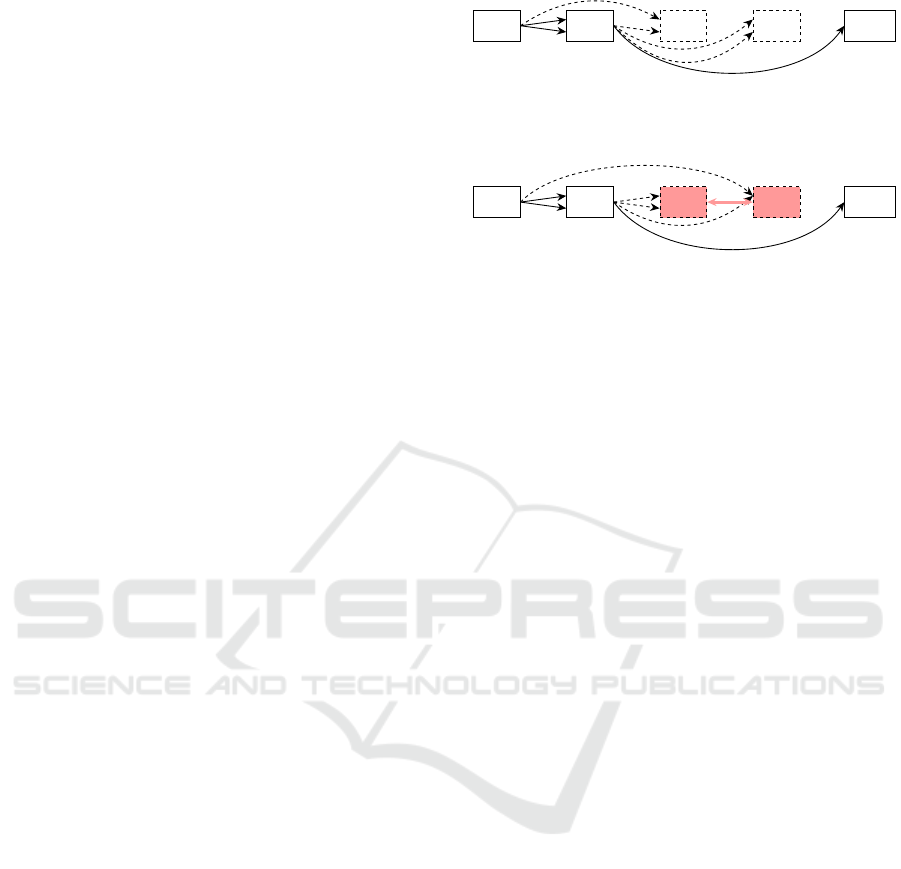
To better illustrate the algorithm of Equidistant-

Reorder, its workings are depicted in Algorithm 2.

Furthermore, Figure 3 shows two example graphs,

with Figure 3a depicting an example graph. Figure 3b

Function Lin-Space:

Data:

• start point s

• end point e

• number of evenly spaced values n

step ←

e − s

;

S ←

i ← 1;

while i ≤ n do

S ← S ∪ bs + i · stepc;

i ← i + 1;

end

Algorithm 1: Generate a set of equidistantly spaced

numbers.

Function Equidistant-Reorder:

A ← all active computational nodes;

A ← all inactive computational nodes;

initialize new genome G with the same

input and output nodes from the old

genome;

s ← |input nodes|;

e ← |input nodes| + |A| + |

A|;

L ← Lin-Space(s, e,|A|);

L ← {s, s + 1, ··· , e} ∩ L;

foreach (a, l) ∈ (A, L) do

G[l] ← a;

end

foreach



˜a,



∈ (

L) do





← ˜a;

end

foreach node ∈ G do

foreach connection

belonging to

node do

update(connection

);

if connection

points to the front

then

mutate connection

;

end

return G;

Algorithm 2: Equidistant-Reorder function.

displays the graph after E-Reorder. Both active nodes

are placed evenly spaced into the new genome, with

the inactive node being assigned to the free position.

ECTA 2023 - 15th International Conference on Evolutionary Computation Theory and Applications

INPUT1

INPUT2

FUNC.

OUTPUT

(a) A graph before E-Reorder. Input and output node are n

, n

and n

. Nodes n

–n

are computational nodes, with FUNC.

being an arbitrary function.

INPUT1

INPUT2

FUNC.

OUTPUT

(b) The graph after a potential E-Reorder, according to Algorithm 2. Node n

must mutate new connections to prevent

connections backwards from the new position of n

to n

Figure 3: A graph deﬁned by a CGP genome, before and after E-Reorder.

4.3 Time Complexity

The modiﬁcations of Equidistant-Reorder compared

to the original Reorder operator from Goldman and

Punch have the same additional runtime complex-

ity (Goldman and Punch, 2013a). In the following,

let N ∈ N

be the number of computational nodes of

the considered CGP graph.

To obtain the set of all active and inactive compu-

tational nodes, O (a ·N) time is needed, where a ∈ N

is the arity of the nodes. Other sets, like L or

L, need

O(N) time. The placing of active and inactive nodes

into a new genome takes only O(N) time, as this only

requires iterating through the sets of active and inac-

tive nodes and their respective new positions once. At

last, the connection genes have to be updated. Never-

theless, this process takes only O(c · N) time by iter-

ating through every computational node and updating

its c connection genes. Please note, a ≡ c, as the high-

est arity a is also the number of connection genes c.

Thus, Equidistant-Reorder needs O(a · N) time,

which is the same as Reorder (Goldman and Punch,

2015).

5 EVALUATION OF E-REORDER

In order to ﬁnd out whether the modiﬁcation we pro-

posed for Reorder truly beneﬁts CGP, we conducted

an empirical study

. This section describes our exper-

Implementation and benchmarks can be found at https:

//github.com/CuiHen/Equidistant Reorder.

imental design. Afterwards, we attempt to answer the

following two questions:

Q1 Which model needs, considering the learning

task, less training iterations: REORDER or E-

REORDER?

Q2 As mentioned in Section 4.1, REORDER may not

reduce the limitation in the search space of CGP.

How does E-REORDER perform compared to RE-

ORDER?

5.1 Experimental Design

In this section, the evaluated CGP conﬁgurations and

utilized benchmarks are presented. Afterwards, we

brieﬂy describe the Bayesian models used to evaluate

and rank different CGP conﬁgurations. With these

models, the performance of multiple conﬁgurations

can be compared by calculating a probability of each

conﬁguration being the best.

5.1.1 Settings of CGP

For our experiments, we compared each combination

of STANDARD, REORDER and E-REORDER in con-

junction with two different mutation strategies: point

mutation and Single. Regarding the hyperparameters,

when the mutation operator Single is used, the only

hyperparameter is the number of nodes N. Thus, we

investigated N ∈ {50, 100, 150, ·· · , 2000} and each N

was tested 75 times with independent repetitions and

different random seeds.

As for the point mutation, the number of nodes N

and the mutation probability p must be determined.

Equidistant Reorder Operator for Cartesian Genetic Programming

For this task, we performed a hyperparameter search

using a Tree-structured Parzen Estimator

. The algo-

rithm performed a total of 100 trials to ﬁnd good hy-

perparameters. For each trial, the conﬁguration was

tested 10 times with independent repetitions and dif-

ferent random seeds. These results were then aver-

aged to obtain a single value. Runs were terminated

when a model is able to solve a benchmark com-

pletely.

Considering the evolutionary algorithms, we uti-

lized a standard (1+4)-ES as described in Section 2.2

for all trainings. Furthermore, to be comparable to

the original evaluations by Goldman and Punch, we

also compared different mutation strategies as already

mentioned above (Goldman and Punch, 2015; Gold-

man and Punch, 2013a). The original works com-

pared two different strategies for the point mutation:

skip and accumulate. However, they did not change

the behaviour of the point mutation but save compu-

tational time only. Furthermore, the authors of the

work (Goldman and Punch, 2015) found no signiﬁ-

cant difference between those two operators. Because

of that, we employed their point mutation strategy of

skip. Offsprings, whose phenotype are equal to the

parents phenotype, are not evaluated. Instead, they

get their parents ﬁtness value assigned.

5.1.2 Problem Set

To evaluate the different settings, we used four

Boolean benchmark problems: 3-bit Parity, 16-4-bit

Encode, 4-16-bit Decode and 3-bit Multiply. In the

following, we will call these Parity, Encode, De-

code and Multiply, respectively. Parity is regarded

as too easy by the Genetic Programming commu-

nity (White et al., 2013). Nevertheless, it is com-

monly used as a benchmark in the literature (Yu

and Miller, 2001; Kaufmann and Kalkreuth, 2020;

Kaufmann and Kalkreuth, 2017). Hence, we also in-

cluded it in our evaluations for ease of comparison.

Encode and Decode are problems with different in-

put and output sizes. At last, Multiply is a compar-

atively hard problem (Walker and Miller, 2008), and

recommended by White et al. (White et al., 2013).

All four benchmarks are used to evaluate REORDER,

too, which is also why we utilized them (Goldman

and Punch, 2013a; Goldman and Punch, 2015).

As we employed four Boolean benchmark prob-

lems, we also trained them with the standard function

set for these problems. They contain the Boolean op-

erators AND, OR, NAND and NOR.

These benchmarks also lead to a standard ﬁtness

For the hyperparameter search, we utilized the Python

library Optuna (Akiba et al., 2019).

function, which is deﬁned by the ratio of correctly

mapped inputs. Let f : {0,1}

→ {0, 1}

be a correct

Boolean mapping for n ∈ N

inputs and m ∈ N

out-

puts. Then, the ﬁtness of an individual g : {0, 1}

→

{0, 1}

, which relates to the learning task f , is deﬁned

as follows:

|{x ∈ {0, 1}

| f (x) = g(x)}|

|{0, 1}

(1)

5.1.3 Bayesian Data Analysis

In search of a good number of nodes for Single, mul-

tiple conﬁgurations were investigated. Furthermore,

to present our ﬁnal results, six different, ﬁnal settings

were compared. In all those cases, each conﬁguration

has to be ranked to ﬁnd the respective best solution.

However, we only considered the number of training

iterations, a unit which can not be negative. Thus,

other common distributions such as Student’s t distri-

butions can not be expected to model the data well.

Hence, we performed a Bayesian data analysis

for

the posterior distributions of our results. The model

to compare the algorithms is based on the Plackett-

Luce model described by Calvo et al. (Calvo et al.,

2018). It allows the computation of a set of ranked

options by estimating the probabilities of each of the

options to be the one with the highest rank.

In addition, in our ﬁnal results, we report for

each conﬁguration the 95 % highest posterior den-

sity intervals (HPDI) of the distribution of µ

con fig

where µ

con fig

is a random variable corresponding to

the respective mean numbers of iterations until solu-

tion. At that, the distribution of µ

con fig

is estimated

by the gamma distribution–based model for compar-

ing non-negative data from cmpbayes (P

atzel, 2023).

Please note, a 95 % HPDI interval [l, u] can be read as

p(l ≤ µ

con fig

≤ u) = 95 %. This means, the probabil-

ity of the algorithms results lying between the bounds

l and u has a probability of 95 %.

On another note, prior sensitivity analyses were

conducted prior to ensure the robustness of all mod-

els. As they always display similar results, ro-

bust and meaningful models are implicated. Finally,

please note that cmpbayes uses Markov Chain Monte-

Carlo sampling to obtain its distributions. There-

fore, the usual checks to ensure convergence and well-

behavedness (trace plots, posterior predictive checks,

R values, effective sample size) were performed. For

more information regarding the models, we refer to

Kruschke and P

atzel (Kruschke, 2013; P

atzel, 2023).

We utilized the Python library cmpbayes (P

atzel, 2023)

for all statistical models.

ECTA 2023 - 15th International Conference on Evolutionary Computation Theory and Applications

5.2 Performance on Training Iterations

As already mentioned, we performed a hyperparame-

ter search and determined the best conﬁguration via a

Plackett-Luce model described by Calvo et al. (Calvo

et al., 2018).

The best results found by the hyperparameter

search can be seen in Table 1. For each benchmark,

the conﬁgurations are sorted from best to worst in de-

scending order. We report the CGP variant and its

mutation operator. Furthermore, we list, with their re-

spective averaged number of iterations needed until

a solution is found, its HPDI, the number of nodes

needed, their mutation rate, the number of active

nodes and the probability of a solution being the best.

For all four benchmarks, our novel variant E-

REORDER probably performed best. For Encode and

Decode, E-REORDER with Single lead to the best re-

sults while Encode and Parity performs best with the

point mutation. This could also mean that we were

not able to ﬁnd the best mutation rate with our hy-

perparameter search. Albeit when looking at the re-

sults for E-REORDER in the context of Encode, the

differences of both mutation operators are almost neg-

ligible. The average number of iterations needed are

almost identical and their HPDI are close, too. Al-

though, according to the Calvo model, the probabili-

ties for E-REORDER with its respective mutation op-

erators are not equal but differ about 5 percentage

points—indicating a preference for the point muta-

tion. On another note, Single needs less nodes to ﬁnd

a solution compared to the point mutation.

Generally, E-REORDER with Single tends to need

the least amount of computational nodes. While

STANDARD with point mutation needs the least

amount of nodes for Multiply, it is also the worst al-

gorithm in this case. This may also be a reason why

E-REORDER needs the least amount of iterations until

a solution is found. With less nodes, the search space

for E-REORDER decreases, too. Hence, it may ﬁnd

a solution faster. Furthermore, with less nodes, CPU

time can be saved with each iteration, as less potential

computations take place.

Interestingly, E-REORDER and REORDER with

the point mutation tend to have similar mutation rates.

Except for Encode, both rates only differ marginally

and varies vastly from STANDARD’s mutation rate. In

our experiments, STANDARD favours a lower muta-

tion rate compared to the other two algorithms, which

could also indicate that REORDER and E-REORDER

favours a higher change in the genotype per mutation.

Another factor for E-REORDER’s better perfor-

mance may be the additional mutations of inactive

nodes. With their reordering, some connection genes

0 20 40 60 80 100

Relative node index in % to the graph's total length

0.0

0.2

0.4

0.6

0.8

1.0

% active during training

Multiply

E-Reorder

Reorder

Standard

Figure 4: Active node distribution of STANDARD, RE-

ORDER and E-REORDER. Each distribution shows the av-

eraged result of 75 aggregated solutions for Multiply.

must be mutated to prevent backward-connections.

This could lead to more genetic drift, which may im-

prove its performance.

5.3 Distribution of Active Nodes

In Section 4.1, we hypothesize a potential limitation

of REORDER and speculate in Section 4.2 that E-

REORDER may further lessen the effects of a posi-

tional bias. Hence, one question we would like to an-

swer is the effect of E-REORDER on the distribution

of active nodes, compared to REORDER and STAN-

DARD. For this task, a visualization of the active node

distribution of the ﬁnal results for all three CGP vari-

ants is given in Figure 4. The x-axis shows the rela-

tive node index in percent, while the y-axis shows the

probability of that node being active.

Please note that we only visualize our ﬁndings for

Multiply, as the other three benchmarks show almost

identical plots and behaviours. In addition, we always

compare the best conﬁgurations found, as reported in

Table 1. Again, we averaged the active node distribu-

tion of 75 independent repetitions with random seeds.

Furthermore, the ﬁgure only depicts the Single muta-

tion strategy, as this was the best mutation operator

for all three CGP variants. Besides, the visualization

for the point mutation strategy shows only marginal

differences compared to Single. At last, as the CGP

variants have different number of nodes, we do not re-

port the actual node indices in Figure 4. Instead, we

report the relative node index in percent to the graphs

total length.

In the context of STANDARD, the positional bias

can be clearly seen. At the beginning of the genome,

nodes have a high probability of being active. How-

ever, after the ﬁrst 30 % of the genome, this probabil-

ity decreases to 10 % or less.

As for REORDER, this variant is able to moder-

ately overcome the bias. While it also contains a drop

in node activity, the decrease is far less pronounced

compared to STANDARD. Furthermore, the probabil-

ity of active nodes increases in the last 10 % of node

indices.

Equidistant Reorder Operator for Cartesian Genetic Programming

Table 1: Best results found for each E-REORDER, REORDER and STANDARD conﬁguration. Algorithms are sorted from best

to worst in descending order. Here, Avg is the average number of iterations until a solution is found; # Nodes is the number of

computational nodes used; p(mut) is the mutation rate; # active is the number of active nodes for this solution; and p(best)

the probability of the solution being the best among the other six.

Variant Mutation Avg HPDI # Nodes p(mut.) # Active p(best)

Parity

E-REORDER Prob. 322 [278, 371] 350 0.081 129 0.26

STANDARD Single 342 [289, 404] 600 — 42 0.23

REORDER Prob. 400 [341, 471] 450 0.085 85 0.21

E-REORDER Single 471 [395,561] 50 — 27 0.16

REORDER Single 739 [606,902] 200 — 57 0.11

STANDARD Prob. 2,524 [2,063, 3,084] 750 0.009 43 0.02

Encode

E-REORDER Prob. 5,294 [4,656, 6,049] 650 0.014 336 0.32

E-REORDER Single 5,296 [4,759,5,908] 150 — 87 0.27

STANDARD Single 6,213 [5,550, 6,947] 200 — 65 0.22

REORDER Prob. 8,642 [7,644, 9,787] 550 0.018 249 0.12

REORDER Single 14,733 [12,786, 16,977] 600 — 258 0.04

STANDARD Prob. 20,378 [17,592, 23,557] 700 0.009 103 0.03

Decode

E-REORDER Single 12,119 [11,174, 13,142] 250 — 145 0.39

E-REORDER Prob. 14,596 [13,154, 16,153] 650 0.008 345 0.26

REORDER Single 15,017 [13,826, 16,295] 700 — 186 0.21

STANDARD Single 23,132 [20,959, 25,482] 400 — 242 0.07

STANDARD Prob. 28,510 [25,868, 31,349] 700 0.009 183 0.04

REORDER Prob. 32,902 [30,227, 35,857] 800 0.003 402 0.03

Multiply

E-REORDER Single 70,304 [59,647, 82,144] 700 — 362 0.41

REORDER Single 90,370 [79,273, 103,286] 750 — 118 0.23

STANDARD Single 129,739 [110,948, 150,742] 700 — 411 0.14

REORDER Prob. 119,426 [104,665, 135,512] 1000 0.013 540 0.13

E-REORDER Prob. 194,044 [163,843, 227,740] 700 0.012 363 0.08

STANDARD Prob. 414,639 [360,719, 472,413] 500 0.007 102 0.02

The distribution for E-REORDER differs com-

pared to the last two CGP variants. For the ﬁrst 5 % of

nodes of graph, the probability for nodes being active

oscillates in the range of [0.2, 1.0]. Afterwards, it ﬂuc-

tuates around a probability of 0.75 % with occasional

spikes in probability. Nevertheless, such ﬂuctuat-

ing behaviour should be anticipated, as E-REORDER

places active nodes equidistantly apart. In addition,

by forcing a uniform distribution of active nodes in

combination with a better ﬁtness value as seen in Sec-

tion 5.2, we believe that we lessened the effects of a

positional bias.

6 CONCLUSION

The existing Reorder operator introduced by Gold-

man and Punch is able to moderately overcome a po-

sitional bias, from which Cartesian Genetic Program-

ming (CGP) suffers (Goldman and Punch, 2013a).

Nonetheless, we theorized that Reorder might have

a small limitation, which may hinder a complete ex-

ploration of the search space. A node may only be

reordered into the new genome when all of its de-

pendencies are satisﬁed—which means that all in-

put nodes must be mapped into the genome before-

hand. This may slightly favour nodes near input

nodes, which could potentially limit Reorders full po-

tential.

ECTA 2023 - 15th International Conference on Evolutionary Computation Theory and Applications

With our novel modiﬁcation to Reorder, called

Equidistant-Reorder, we are able to evade the limi-

tation of Reorder. The algorithm works by reordering

active nodes equidistantly apart throughout the whole

genome. As a result, CGP with Equidistant-Reorder

is able to ﬁnd a solution for a given problem in less

iterations compared to the CGP baseline or with the

Reorder extension. In most cases, the total number of

nodes needed to train CGP is reduced, too.

As for future work, different reorder strategies

could be examined as we only focused on equidis-

tant spacing. It would also be possible to apply a

uniform distribution instead of enforcing an equidis-

tant distance. Another interesting aspect would be to

move all or the majority of active nodes to the end of

the genome. Then, there are almost no nodes with a

higher probability of becoming active. As all active

nodes are at the end of the genome, each node is able

to mutate a connection to an arbitrary node behind. It

may lead to less positional bias, too, but could also

lead to other potential problems.

ACKNOWLEDGEMENTS

The authors would like to thank the German Federal

Ministry of Education and Research (BMBF) for sup-

porting the project SaMoA within VIP+.

REFERENCES

Akiba, T., Sano, S., Yanase, T., Ohta, T., and Koyama, M.

(2019). Optuna: A next-generation hyperparameter

optimization framework. In Proceedings of the 25th

ACM SIGKDD International Conference on Knowl-

edge Discovery and Data Mining.

Bentley, P. J. and Lim, S. L. (2017). Fault tolerant fusion

of ofﬁce sensor data using cartesian genetic program-

ming. In 2017 IEEE Symposium Series on Computa-

tional Intelligence (SSCI), pages 1–8. IEEE.

Calvo, B., Ceberio, J., and Lozano, J. A. (2018). Bayesian

inference for algorithm ranking analysis. In Proceed-

ings of the Genetic and Evolutionary Computation

Conference Companion, GECCO ’18, page 324–325,

New York, NY, USA. Association for Computing Ma-

chinery.

Froehlich, S. and Drechsler, R. (2022). Unlocking approxi-

mation for in-memory computing with cartesian ge-

netic programming and computer algebra for arith-

metic circuits. it - Information Technology, 64(3):99–

107.

Goldman, B. W. and Punch, W. F. (2013a). Length bias

and search limitations in cartesian genetic program-

ming. In Proceedings of the 15th Annual Conference

on Genetic and Evolutionary Computation, GECCO

’13, page 933–940, New York, NY, USA. Association

for Computing Machinery.

Goldman, B. W. and Punch, W. F. (2013b). Reducing

wasted evaluations in cartesian genetic programming.

In Genetic Programming, pages 61–72, Berlin, Hei-

delberg. Springer Berlin Heidelberg.

Goldman, B. W. and Punch, W. F. (2015). Analysis of

cartesian genetic programming’s evolutionary mech-

anisms. IEEE Transactions on Evolutionary Compu-

tation, 19(3):359–373.

Harding, S., Leitner, J., and Schmidhuber, J. (2013). Carte-

sian Genetic Programming for Image Processing,

pages 31–44. Springer New York, New York, NY.

Harding, S. L., Miller, J. F., and Banzhaf, W. (2011). Self-

Modifying Cartesian Genetic Programming, pages

101–124. Springer Berlin Heidelberg, Berlin, Heidel-

berg.

Huang, W., He, P., Yan, Z., and Wu, H. (2022). An efﬁcient

MRI impulse noise multi-stage hybrid ﬁlter based on

cartesian genetic programming. In Advances in Natu-

ral Computation, Fuzzy Systems and Knowledge Dis-

covery, pages 95–106, Cham. Springer International

Publishing.

Kalkreuth, R. (2022). Phenotypic duplication and inversion

in cartesian genetic programming applied to boolean

function learning. In Proceedings of the Genetic and

Evolutionary Computation Conference Companion,

GECCO ’22, page 566–569, New York, NY, USA. As-

sociation for Computing Machinery.

Kaufmann, P. and Kalkreuth, R. (2017). An empirical study

on the parametrization of cartesian genetic program-

ming. In Proceedings of the Genetic and Evolutionary

Computation Conference Companion, GECCO ’17,

page 231–232, New York, NY, USA. Association for

Computing Machinery.

Kaufmann, P. and Kalkreuth, R. (2020). On the parame-

terization of cartesian genetic programming. In 2020

IEEE Congress on Evolutionary Computation (CEC),

pages 1–8.

Kruschke, J. K. (2013). Bayesian estimation supersedes the

t test. Journal of Experimental Psychology: General,

142(2):573.

Leitner, J., Harding, S., F

orster, A., and Schmidhuber,

J. (2012). Mars terrain image classiﬁcation using

cartesian genetic programming. In Proceedings of

the 11th International Symposium on Artiﬁcial Intel-

ligence, Robotics and Automation in Space, i-SAIRAS

2012, pages 1–8. European Space Agency (ESA).

Manazir, A. and Raza, K. (2022). pcgp: A parallel imple-

mentation of cartesian genetic programming for com-

binatorial circuit design and time-series prediction. In

2022 International Conference on Electrical, Com-

puter and Energy Technologies (ICECET), pages 1–4.

Margraf, A., Stein, A., Engstler, L., Geinitz, S., and Hah-

ner, J. (2017). An evolutionary learning approach to

self-conﬁguring image pipelines in the context of car-

bon ﬁber fault detection. In 2017 16th IEEE Interna-

tional Conference on Machine Learning and Applica-

tions (ICMLA), pages 147–154. IEEE.

Equidistant Reorder Operator for Cartesian Genetic Programming

Miller, J. F. (1999). An empirical study of the efﬁciency of

learning boolean functions using a cartesian genetic

programming approach. In Proceedings of the 1st An-

nual Conference on Genetic and Evolutionary Com-

putation - Volume 2, GECCO’99, page 1135–1142,

San Francisco, CA, USA. Morgan Kaufmann Publish-

ers Inc.

Miller, J. F. (2011). Cartesian Genetic Programming.

Springer Berlin Heidelberg, Berlin, Heidelberg.

Miller, J. F. (2020). Cartesian genetic programming: its sta-

tus and future. Genetic Programming and Evolvable

Machines, 21(1):129–168.

Payne, A. J. and Stepney, S. (2009). Representation and

structural biases in cgp. In 2009 IEEE Congress on

Evolutionary Computation, pages 1064–1071.

atzel, D. (2023). cmpbayes. Available at:

https://github.com/dpaetzel/cmpbayes, commit =

4de0abc37ee28b35267db173d32bb96ca9e69236.

Suganuma, M., Kobayashi, M., Shirakawa, S., and Nagao,

T. (2020). Evolution of Deep Convolutional Neu-

ral Networks Using Cartesian Genetic Programming.

Evolutionary Computation, 28(1):141–163.

Torabi, A., Shariﬁ, A., and Teshnehlab, M. (2022). Us-

ing cartesian genetic programming approach with new

crossover technique to design convolutional neural

networks. Neural Processing Letters.

Turner, A. J. and Miller, J. F. (2015). Neutral genetic

drift: an investigation using cartesian genetic pro-

gramming. Genetic Programming and Evolvable Ma-

chines, 16(4):531–558.

Vassilev, V. K. and Miller, J. F. (2000). The advantages

of landscape neutrality in digital circuit evolution. In

Evolvable Systems: From Biology to Hardware, pages

252–263, Berlin, Heidelberg. Springer Berlin Heidel-

berg.

Walker, J. A. and Miller, J. F. (2004). Evolution and acquisi-

tion of modules in cartesian genetic programming. In

Genetic Programming, pages 187–197, Berlin, Hei-

delberg. Springer Berlin Heidelberg.

Walker, J. A. and Miller, J. F. (2008). The automatic ac-

quisition, evolution and reuse of modules in cartesian

genetic programming. IEEE Transactions on Evolu-

tionary Computation, 12(4):397–417.

White, D., Mcdermott, J., Castelli, M., Manzoni, L., Gold-

man, B., Kronberger, G., Ja

skowski, W., O’Reilly, U.-

M., and Luke, S. (2013). Better gp benchmarks: Com-

munity survey results and proposals. Genetic Pro-

gramming and Evolvable Machines, 14:3–29.

Wilson, D. G., Miller, J. F., Cussat-Blanc, S., and Luga,

H. (2018). Positional cartesian genetic programming.

arXiv preprint arXiv:1810.04119.

Yu, T. and Miller, J. (2001). Neutrality and the evolvability

of boolean function landscape. In Genetic Program-

ming, pages 204–217, Berlin, Heidelberg. Springer

Berlin Heidelberg.

ECTA 2023 - 15th International Conference on Evolutionary Computation Theory and Applications