Comparative Analysis of Segmentation Techniques for Reticular

Structures

Francisco J. Soler

1 a

, Luis M. Jim

enez

1 b

, David Valiente

1 c

, Luis Pay

1 d

and

Oscar Reinoso

1,2 e

Engineering Research Institute of Elche (I3E), Miguel Hernandez University, Elche, Spain

ValgrAI: Valencian Graduate School and Research Network of Artiﬁcial Intelligence, Valencia, Spain

Keywords:

Plane Segmentation, Point Clouds, Region Growing, RANSAC, Neural Networks, Climbing Robots.

Abstract:

Nowadays neural networks are widely used for segmentation tasks and there is a belief that these approaches

are synonymous of advances and improvements. This article aims to compare the performance of a neural

network, trained in our previous work, and an algorithm which is speciﬁcally designed for the segmentation

of reticular structures. As shown in this paper, in certain cases it is feasible to use conventional techniques

outside the paradigm of artiﬁcial intelligence achieving the same performance. To prove this, in this article a

quantitative and qualitative comparative analysis is carried out between an ad hoc algorithm for segmenting

reticular structures and the model of neural network that provided the best results in our previous work in this

task. Established techniques such as Random Sample Consensus (RANSAC) and region growing have been

used to implement the proposed algorithm. For the quantitative analysis, standard metrics such as precision,

recall and f1-score are used. These metrics will be calculated with a self-generated dataset, consisting of

a thousand point clouds that were generated automatically in the previous work. The studied algorithm is

tailor-made for this database. For reproducibility, code and datasets are provided at https://github.com/Urwik/

rrss grnd ﬁlter.git.

1 INTRODUCTION

Most existing large-scale buildings use lattice systems

as structural elements due to their outstanding me-

chanical properties. These properties enable them to

withstand high loads, achieve a balanced distribution

of forces, exhibit high rigidity, and demonstrate efﬁ-

ciency in terms of material usage.

Due to these excellent properties, lattice structures

(Figure 1) are widely used in high-voltage transmis-

sion lines, tower cranes, bridges, and other large-scale

infrastructures. Typically, these structures are assem-

bled using metallic bodies, in most cases these bodies

are composed of ﬂat surfaces, as seen in the case of

transmission lines. In other cases these structures can

be built with cylindrical parts.

As a general rule, these infrastructures respond ad-

equately to adverse weather conditions and hostile en-

https://orcid.org/0009-0006-7396-6596

https://orcid.org/0000-0003-3385-5622

https://orcid.org/0000-0002-2245-0542

https://orcid.org/0000-0002-3045-4316

https://orcid.org/0000-0002-1065-8944

vironments, nevertheless require regular maintenance

and inspection. A constantly evolving ﬁeld of re-

search involves the use of climbing robots to perform

these types of tasks (Fang and Cheng, 2023). Climb-

ing robots are devices known for their ability to move

and operate on various surfaces, both horizontal and

vertical, such as walls, ceilings, or metallic structures.

Additionally, they can perform multiple inspection or

maintenance tasks in complex environments that are

difﬁcult to access and pose signiﬁcant risks to human

operators, who may be exposed to various hazards

such as falls or electric shocks.

These types of inspections and maintenance tasks

have been carried out by aerial robots in recent years

((Akahori et al., 2016), (Jung et al., 2019)). However,

quite often this type of robotic platform is unable to

complete such tasks due to its limitation in accessing

internal areas of the structures.

In order to carry out such tasks effectively, it is

necessary to have a proper environmental perception.

One of the sensors most widely used today for sensing

surroundings are the so-called LiDAR. These sensors,

widely used in numerous applications today, such as

Soler, F., Jiménez, L., Valiente, D., Payá, L. and Reinoso, Ó.

Comparative Analysis of Segmentation Techniques for Reticular Structures.

DOI: 10.5220/0012177100003543

In Proceedings of the 20th International Conference on Informatics in Control, Automation and Robotics (ICINCO 2023) - Volume 1, pages 413-423

ISBN: 978-989-758-670-5; ISSN: 2184-2809

413

Figure 1: Example of reticular structure used in an indus-

trial building.

localization (Liu et al., 2022), map building (Zhou

et al., 2021), object detection and segmentation (Zhu

et al., 2021), provide excellent range information.

Their high accuracy in providing detailed information

about the spatial distribution of the environment has

made this type of sensor widely used for localisation

and navigation in robotics in recent years.

A key aspect for accurate navigation is the clear

identiﬁcation of ﬂat surfaces in the surrounding en-

vironment (Xu et al., 2020). The presence of planes

in the structure allows us to build a parametric rep-

resentation of it, enabling a lightweight environment

model. Consequently, detecting these types of ele-

ments in the environment is a task of interest for nav-

igation in lattice structures.

Providing a climbing robot with a LiDAR sen-

sor allows it to know the spatial distribution of the

surrounding environment. Combined with the ability

to identify planar surfaces, it may constitute an ideal

solution to address navigation tasks in lattice struc-

tures, where virtually all components are made up of

planes. By combining the information from the Li-

DAR sensor and the detection of ﬂat surfaces, the

robot can effectively navigate and interact with the

Figure 2: Example of captured cloud by the simulated sen-

sor.

structure, leveraging its knowledge of the planar el-

ements within the environment.

Indeed, LiDAR sensors often capture a large

amount of information, sometimes more than neces-

sary (Figure 2). Therefore, it becomes crucial to re-

move undesired data. At ﬁrst, the main objective to

enable the navigation of the robotic platform through-

out this type of structures, is to identify from all the

information provided by the available sensory sys-

tems, the information relating only to the structure,

being necessary to identify which part of the informa-

tion belongs to it and which does not. This task could

be deﬁned as a per point classiﬁcation or a segmenta-

tion of the original information into certain classes.

In recent years, we can ﬁnd related works that

employ artiﬁcial intelligence systems and algorithms

to address this problem. Thus, we ﬁnd some works

on plane segmentation with neural networks such as

(Yang and Kong, 2020) or (Lee and Jung, 2021).

In these works, neural networks are used to iden-

tify planes in indoor and outdoor environments (ur-

ban environments) respectively. However, these envi-

ronments differ signiﬁcantly from the target environ-

ments of our work, which is why in previous works

in the research group we approached this task with a

segmentation proposal using speciﬁc neural networks

(Soler et al., 2023).

Additionally, there are many methods for plane

identiﬁcation with algorithms outside the artiﬁcial in-

telligence paradigm as in (Su et al., 2022). It proposes

a two-step segmentation, a ﬁrst stage where planes

are selected by region growing and a second stage

where the border points between two planes are clas-

siﬁed, where the region growing algorithm is not able

to work correctly. In (Gaspers et al., 2011) they sim-

ilarly use a two-stage segmentation but over multiple

resolutions. They extract for each resolution key fea-

tures based on the normals named surfels. These sur-

fels are intended to be associated with planes at lower

resolutions. Those surfels that are not associated with

any known plane are attempted to be grouped accord-

ing to their coplanarity using the Hough transform.

On the other hand, RANSAC is applied to the sets of

surfels that have been associated with the same plane

at lower resolutions to improve accuracy. Once the

maximum resolution is reached, nearby coplanar seg-

ments are identiﬁed and merged into a single plane.

The algorithm proposed in this study is similar

to the ones mentioned above, as it employs a two-

stage strategy, but unlike the previous ones (segment-

ing the point cloud provided by the LiDAR sensor

into multiple ﬂat sets) its objective is to split the point

cloud only into two sets, structure and non-structure.

For this purpose, a coarse classiﬁcation by RANSAC

ICINCO 2023 - 20th International Conference on Informatics in Control, Automation and Robotics

414

is used and then a region growing procedure is per-

formed to improve the result.

The aim of this article is to evaluate the per-

formance of neural networks against the application

of such speciﬁc algorithm for segmenting reticular

structures in a speciﬁc environment. To do so, we

will compare our previous work, (Soler et al., 2023),

with a proposed application-speciﬁc algorithm using

a dataset that contains point clouds obtained from

reticular structures.

To provide a clear overview, this articles is divided

into the following parts. Second section (2) brieﬂy re-

counts the previous work in order to put the reader in

context for further comparison. Section 3 explores the

proposed method for segmenting the lattice structures

of our database and discusses all its steps. Section

4 presents the conducted experiments. Then, Sec-

tion 5 develops a comparative analysis between the

segmentation of reticular structures using neural net-

works and conventional approaches. Finally, Section

6 discusses some brief reﬂections about the obtained

results.

2 PREVIOUS WORK

In this section, we provide a brief overview of the fun-

damental idea of our previous work. In previous stud-

ies (Soler et al., 2023), an speciﬁc training of neu-

ral networks was made to identify reticular structures

based on environment information provided by a Li-

DAR sensor.

Reticular structures are interconnected systems by

rigid joints forming a three-dimensional lattice con-

ﬁguration. This type of system can be found in a mul-

titude of infrastructures, such as bridges, buildings,

electricity pylons or cranes, and is normally made by

metallic elements composed by multiple ﬂat surfaces.

The aforementioned work was carried out with the

purpose of being implemented in the HyReCRo (Pei-

dro et al., 2015) robot. This series-parallel climb-

ing robot has ten degrees of freedom (DOF) and has

the ability to navigate through metallic structures by

using a magnetic adhesion mechanism based on me-

chanically switched permanent magnets.

2.1 Dataset Generation

One of the ﬁrst challenges to be solved in order to

meet the objective of previous work was the lack of

training dataset.

There are recent studies on the use of simulators

for the automatic generation of labelled datasets. In

(Sanchez et al., 2019) Gazebo Simulator is used to

generate labelled 3D scans of natural environments,

but it has a limitation when it comes to generating

large datasets, as the position of the sensor has to be

indicated by the user. In a more autonomous way,

in (Wang et al., 2019) a modiﬁcation of the CARLA

simulator (Dosovitskiy et al., 2017) is used to gener-

ate driving LiDAR point clouds with per point auto-

matic labels during the movement of a vehicle. More-

over, there are studies that merge real and synthetic in-

formation such as (Fang et al., 2018), where similar to

the work mentioned above its objective is to generate

driving data. To achieve that, they use a static labelled

point cloud as a background and introduce synthetic

elements, like cars or people, with pre-deﬁned labels

in order to obtain a more realistic representation of

the environment.

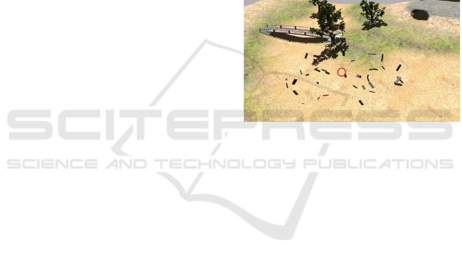
Figure 3: Example of environment used for training. Red

circle indicates the position of the sensor.

The works mentioned above mainly focus on au-

tonomous driving navigation and segmentation of

such environments. To address the segmentation of

lattice structures where the environment differs sig-

niﬁcantly from the previous ones, we have developed

a plugin in Gazebo Simulator. Similar to (Sanchez

et al., 2019), it uses this simulation software to gener-

ate labelled datasets automatically, with the advantage

that the position of the sensor and the elements of the

environment change automatically, enabling the gen-

eration of large databases.

The training database was conformed by ten thou-

sand point clouds simulating the properties of a real

LiDAR sensor (Ouster OS1-128 channels). Each

measure is taken from the sensor origin and the sensor

pose is set randomly around the environment. With

the objective of generalising the database for a vari-

ety of lattice structures, the training dataset is formed

using environments composed of parallelepipeds and

elements such as trees and soil modelling a real envi-

ronment (Figure 3).

In the same way as for the training data, the eval-

uation dataset (which is the one used to evaluate the

metrics in this paper) has been generated automati-

Comparative Analysis of Segmentation Techniques for Reticular Structures

415

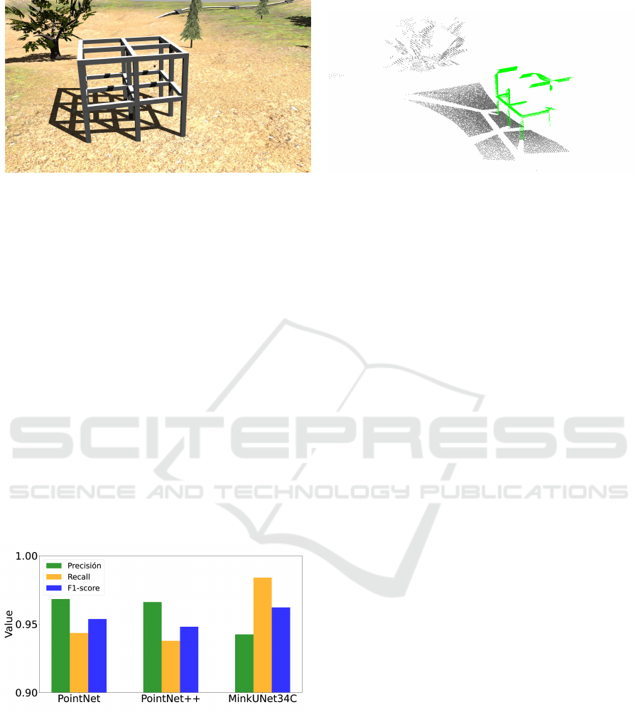
(a) Example of the evaluation environment. (b) Example of the point cloud generated with automatic la-

bels.

Figure 4: Example of the evaluation dataset.

cally. It is composed of 904 point clouds and with a

lattice structure model instead of parallelepipeds. A

representation of the evaluation environment and the

simulated data are shown in the Figure 4.

Different neural network architectures were

trained and analysed for reticular structure segmenta-

tion, PointNet (Qi et al., 2016), PointNet++ (Qi et al.,

2017) and MinkUNet34C (Choy et al., 2019). The

best results were obtained with the MinkUNet34C ar-

chitecture, which uses the MinkowskiEngine to per-

form 3D convolutions in a sparse way, only on those

points that contain information. The latter architec-

ture shows better results in terms of recall and f1 score

than the others as shown in Figure 5, therefore it has

been selected as the best model for comparison.

Their results are discussed and compared in fur-

ther detail with the algorithm presented in the present

article in Section 5.

Figure 5: Metrics obtained in previous work.

3 PROPOSED ALGORITHM

The algorithm proposed in this study is structured in

two steps. The ﬁrst step performs a coarse classi-

ﬁcation, identifying the ground plane and elements

close to it. Secondly, a process is run in which the

classiﬁcation is reﬁned. This method adopts well-

known algorithms in the literature for plane segmen-

tation and identiﬁcation such as region growing or

Random Sample Consensus (RANSAC) with the aim

of classifying points into two classes, structure and

non-structure.

It is important to notice that this algorithm has

been speciﬁcally designed to work in the environ-

ments that have been generated for the test dataset in

our previous work. While deﬁning its behaviour, it is

taken into consideration that within the sensor read-

ing there will be a large number of points belonging

to the ground, in addition to the fact that these occupy

a large area of the environment. Figure 6 shows a

ﬂowchart that describes the process followed to com-

plete the segmentation. The implementation of this

work relies on the Point Cloud Library (PCL) (Rusu

and Cousins, 2011) library to perform the point cloud

processing. The following subsections describe each

of its stages in more detail.

To reduce the computational cost of the algorithm,

a two-stage approach is adopted. Based on the pre-

liminar experiments, the highest computational cost

of the algorithm is due to the normal estimation, a

process that consumes about 80% of the total execu-

tion time of the algorithm. If the ﬁne classiﬁcation

step is used directly, it would be necessary to estimate

the normals of the entire cloud, in addition to having

to calculate and evaluate the eigenvalues of a larger

number of ensembles. Such an approach would re-

quire on average 20% more runtime per cloud to ob-

tain the same results.

3.1 Coarse Segmentation

In the initial stage of the algorithm a coarse clas-

siﬁcation is performed to extract the ground points.

This stage involves Voxel ﬁltering followed by the ex-

traction of the largest plane in the environment using

RANSAC.

ICINCO 2023 - 20th International Conference on Informatics in Control, Automation and Robotics

416

Coarse Ground

Density Filter

Original

Point Cloud

Voxel

Filter

RANSAC

Largest Plane

Region Growing

Eval

EigenValues

Coarse Truss

Final GroundFinal Truss

Yes

Fine Segmentation

Coarse Segmentation

Figure 6: Flowchart of the proposed algorithm.

Since RANSAC selects the best plane candidate

based on the number of inliers, if there are areas with

high point density, RANSAC tends to select planes in

these areas. To avoid this problem, Voxel ﬁltering is

ﬁrst applied, a process by which the point density is

homogenised across the entire cloud, thus favouring

the extraction of the largest plane (ground plane).

In order to cover as many ground points as pos-

sible, a high threshold is established to obtain the

largest plane, around 0.5 metres, thus avoiding slopes

in the terrain.

3.2 Fine Segmentation

Coarse classiﬁcation produces a smaller cloud con-

taining ground points as well as points close to it

within a certain threshold. On this reduced cloud, a

more accurate classiﬁcation is applied. The idea of

this stage is to split the cloud into planar clusters and

to classify them according to their size.

In order to segment the different planar clusters,

region growing based on the normals is applied. The

clustering process is based on the similarity of the

normals of nearby points, so the estimation of these

features is a very important aspect in the resultant

clusters.

In the following subsections, the normal estima-

tion for each point and the decision criteria for cluster

ﬁltering are further discussed.

3.2.1 Normal Estimation

As mentioned in the previous section, normal esti-

mation is a key component in establishing correct

planar clusters. The normal estimation function im-

plemented in PCL consists of computing the eigen-

values and eigenvectors over the neighbourhood of

each point, where the eigenvector associated with the

smallest eigenvalue is considered the normal vector of

the point. Eigenvalues and eigenvectors are obtained

by principal component analysis (PCA) on the covari-

ance matrix for each point and its neighbourhood en-

vironment.

This matrix (C ) follows the formulation indicated

in Equation 1, where k is the number of neighbors,

p is the centroid of the neighbor set, λ

is the eigen-

value, and

⃗

is the eigenvector for j.

C =

∑

i=1

·(p

− p) · (p

− p)

C ·

⃗

= λ

⃗

, j ∈ {0,1, 2}

(1)

The normal estimation method described in the

previous paragraph requires the selection of a set of

neighbouring points to fulﬁl its task. The imple-

mentation of the library allows two exclusive options

for this purpose: to select all points located within

a sphere of deﬁned radius, or to select those closest

points with a limit in number.

Depending on the neighbour selection method, the

eigenvectors and eigenvalues can differ signiﬁcantly.

An example of this can be seen in Figure 7 where the

point cloud is represented as a function of its curva-

ture (2), deﬁned as the coefﬁcient between the small-

est eigenvalue and the sum of all eigenvalues. In Fig-

ure 7(a) neighbours are selected by radius and in Fig-

ure 7(b) by nearest neighbours.

Curvature =

+ λ

(2)

Comparative Analysis of Segmentation Techniques for Reticular Structures

417

(a) By radius

(b) By neighbours

Figure 7: Point clouds displayed by its curvature.

Based on the conducted experiments, it has been

concluded that the estimation of the normal vector of

each point is more accurate when a certain number of

close neighbours are used. The normal estimation by

radius is highly erroneous in areas with a low density

of points, i.e. there are not enough points in the indi-

cated radius to estimate the normal vector. In contrast,

the calculation of curvature, which is somewhat in-

dicative of point spread, is more accurate when neigh-

bour selection by radius is used, as seen in Figure 7,

where in the radius selection method, points with high

curvature correspond to the cutting edges of the dif-

ferent planes of the structure. The curvature value

is important since, as described below, it is used as

a termination criteria for growing regions. As indi-

cated in (Pauly et al., 2002), if we look at equation

(2), the maximum curvature value will be λ

max

= 1/3

which occurs when λ

= 1, since λ

≤ λ

and

0−2

∈ {0, 1}.

This means that small values of curvature indicate

that the points are poorly sparse along the smallest

eigenvector (most of the points fall on a plane) and

values close to 1/3 in curvature mean that the points

are uniformly sparse throughout the selected neigh-

bourhood space.

3.2.2 Region Growing

The region growing method is a frequently employed

approach for detecting and grouping data sets into

cohesive regions. It operates on the fundamental

premise that neighboring points exhibiting similar at-

tributes should be grouped together.

In this study, the existing implementation in the

PCL library is used, which facilitates region growth

based on the normal vector associated with each

point. Primarily, it is imperative to estimate the nor-

mals and their corresponding curvature. Once this

estimation is accomplished, the initial seed point is

selected based on the lowest curvature value across

the entire point cloud. Subsequently, the cluster’s size

expands by incorporating neighboring points that sat-

isfy speciﬁc criteria. In order to include a new point

in the set, two conditions must be satisﬁed. The ﬁrst

condition involves assessing the angular disparity be-

tween the point’s normal and the initial seed’s nor-

mal. If the difference falls below a speciﬁc threshold,

the new point is incorporated into the set. The sec-

ond condition entails examining the curvature of the

newly added points. If the curvature is below a certain

threshold, these points become new seeds for further

expansion of the set. This growth process continues

until no more seeds are available, indicating the com-

pletion of set expansion.

3.2.3 Eigenvalues Evaluation

To determine whether a region belongs to the struc-

ture or not, the eigenvalues and eigenvectors are em-

ployed as indicators. These properties are derived

through a principal component analysis conducted on

the covariance matrix of the local neighborhood sur-

rounding a speciﬁc point, similar to the method de-

scribed in the preceding section for normal estima-

tion.

The algorithm has been assessed with three dif-

ferent variations, differing in the approach utilized to

determine whether a cluster of points belongs to the

structure or not. These variations focus on distinct

methods of utilizing eigenvalues or eigenvectors for

this discrimination process.

By Ratio. This particular variant builds upon exist-

ing knowledge of the structure, assuming that struc-

tural planes exhibit an elongated and slender geome-

try. Taking this into account, this variant relies solely

on the ratio between the two largest eigenvalues (re-

ferred to as the ”ratio” in Equation 3) to calculate

a value representing the length-to-width ratio of the

candidate set. This value is then utilized to determine

the classiﬁcation of the cluster in question.

ICINCO 2023 - 20th International Conference on Informatics in Control, Automation and Robotics

418

ratio =

(3)

By Module. Applying a similar methodology to the

previous variant, having prior knowledge of the bar-

like geometry of the structure enables ﬁltering based

on the projection module of the farthest point along

its principal axes. Thresholds are then deﬁned for

the two dimensions of the plane formed by the set of

points.

Groups of points exceeding the speciﬁed thresh-

olds (maximum length and width of the structural el-

ements) are excluded from the classiﬁcation as part of

the structure.

Hybrid. In the ﬁnal variant, a combination of the

two preceding approaches is employed, incorporating

both the module ﬁltering and the ratio-based classiﬁ-

cation. This integrated method yields the most favor-

able outcomes, as evident from the results presented

in Table 1.

3.2.4 Density Filter

Lastly, considering the proximity of the robot and sen-

sor to the structure, it is expected that areas belong-

ing to the structure will exhibit a higher point den-

sity, while the ground and surrounding environment

will show lower density. Taking advantage of this ob-

servation, the ﬁnal step aims to eliminate remaining

spurious points in the environment, retaining only the

points corresponding to the structure. This step effec-

tively ﬁlters out outlier points, resulting in a represen-

tation that solely encompasses the desired structure.

3.3 Limitations

It is important to emphasize that the algorithm is

speciﬁcally tailored for the available dataset, which

encompasses a wealth of information regarding the

environment and the ground. This dataset is ob-

tained through a realistic simulation of the commer-

cial Ouster OS1 LiDAR sensor, ensuring that the gen-

erated data adheres to the sensor’s speciﬁcations. The

conﬁguration of the simulated sensor includes a res-

olution of 512x128 points, a maximum range of 30

meters, vertical and horizontal ﬁelds of view of 45

degrees and 360 degrees respectively. Additionally,

the dataset incorporates Gaussian noise with a mean

of zero and a standard deviation of 0.008 meters.

The extensive ﬁelds of view and range of the sensor

enable comprehensive information capture from the

ground and surrounding environment, enabling the

algorithm’s initial stage to successfully identify the

ground plane.

4 EXPERIMENTS

The hardware used for the experiments is as follows.

An NVIDIA RTX3090 graphics card in the case of the

neural network. An Intel i7-10700 processor for all

variants of the proposed ad hoc algorithm. The results

obtained during the experiments are shown in Table

1, where the metrics evaluated (Section 5.1) are listed

together with the execution time in milliseconds.

4.1 Ratio

Experiments with this algorithm variant have been

performed with a threshold for the ratio given by the

prior knowledge of the structure, taken as the quotient

between the width of the beams and the height men-

tioned in Section 3.1 by which the points close to the

estimated ground plane are selected. Assessing clus-

ters with this variant yields poor results because it is

not able to classify correctly large clusters belonging

to the ground, whose elongated proportions are simi-

lar to those of the beams.

4.2 Module

For this approach, the threshold has been taken as the

height above which points close to the ground are se-

lected to obtain a coarse classiﬁcation. This distance

is taken as the threshold since it is the maximum bar

length visible after coarse classiﬁcation. The results

of this variant are considerably better than the previ-

ous one, since it is able to identify the clusters ob-

tained according to their size, thus overcoming the

problem of the previous method. Despite this, it is

possible that the clusters meet the size requirement,

but not the ratio requirement (Figure 8).

Figure 8: Example of a cluster that can not be correctly

classiﬁed by its module.

Comparative Analysis of Segmentation Techniques for Reticular Structures

419

Table 1: Evaluated results in the comparison. W/O = without.

Precision Recall F1-Score TP FP TN FN

Execution Time

(ms)

MinkUNet34C 0,9425 0,9840 0,9622 10213 623 14006 158 45

RATIO 0,6972 0,9658 0,7961 10024 5133 9492 349 62

MODULE 0,9920 0,9645 0,9775 10007 70 14555 366 72

HYBRID 0,9922 0,9643 0,9775 10004 67 14558 368 72

W/O Coarse Seg 0,9952 0,4422 0,6123 4587 22 14603 5786 89

W/O Fine Seg 0,9935 0,9575 0,9744 9940 52 14574 433 31

4.3 Hybrid

The same thresholds are used for this variant as for

the previous ones. The hybrid ﬁlter allows us to take

into account those clusters that meet the modulus re-

quirement but do not meet the ratio requirement, as

in the example in Figure 8. This result is not signif-

icant in the evaluated metrics as it hardly appears in

the available data (only when there are certain occlu-

sions). In Figure 8, an example of this type of situa-

tion is shown, where a cluster that meets the module

requirements, does not meet the ratio requirements

and therefore has to be discarded.

4.4 Without Coarse Segmentation

This experiment has been carried out with the hy-

brid method as it is the most complete for the given

task. Applying directly a ﬁne classiﬁcation, i.e. re-

gion growing to segment the input cloud does not pro-

vide the best results. This fact is supported by the

results in Table 1.

In the later one, it can be seen that in this case a

good precision is achieved, which implies that those

points identiﬁed as structure are indeed structure. On

the other hand, its recall is only close to 50%, which

means that only this percentage of the structure can

be identiﬁed.

This method is mainly based on the accurate esti-

mation of the clusters by region growing, which de-

pends on a multitude of parameters and requires an

exhaustive adjustment of these for an ideal perfor-

mance. By evaluating each of the clusters formed us-

ing the decision criteria (hybrid criteria in this case),

the sets are classiﬁed as structure and non-structure.

In order to obtain better results with this method, it

would be necessary to carry out an improvement pro-

cess to adjust the parameters of normal estimation and

region growing.

Besides, in this case it is necessary to adjust the

thresholds used in the previous experiments, setting as

module the maximum length of the bars of the struc-

ture (since they are complete and not trimmed) and

consequently the ratio with mentioned length.

4.5 Without Fine Segmentation

A further studied scenario is the use of the algo-

rithm without the ﬁne classiﬁcation section. Its ac-

curacy is very high, because with ground voxelization

and RANSAC we are able to accurately identify the

ground plane, as these are structures that rise from

the ground, everything above a certain height is eas-

ily classiﬁed as structure. By using this method, the

execution time can be reduced by almost half.

Despite these facts, this method is not able to iden-

tify the points where the structure meets the ground

and discards all of them. Since the point density in

these areas of the structure is not very high and their

number is very small compared to the rest, the metrics

evaluated are not affected to any large extent.

However, in order to obtain the best results, the

ﬁne classiﬁcation stage is proposed to meet the needs

of identifying areas where the structure meets the

ground. Although its behaviour is far from ideal due

to the reduced density of points in these areas, its

use implies an improvement in certain cases. An ex-

ample of this type of situation is shown in Figure 9,

where the ﬁne segmentation stage is able to identify

the points corresponding to the elements of the struc-

ture in contact with the ground, improving the ﬁnal

classiﬁcation. In this case, the use of this type of clas-

siﬁcation with respect to the hybrid method means an

increase in precision, as expected, but a reduction in

recall of around 4%.

4.6 Density Filter

Applying the density ﬁlter to the initial cloud or after

the proposed methods has also been evaluated. It has

been observed that the best results of the algorithm are

obtained when the density ﬁlter is used last. This may

be due to the larger amount of information available

to the ﬁne and coarse stages to operate.

ICINCO 2023 - 20th International Conference on Informatics in Control, Automation and Robotics

420

(a) Without Fine Segmentation

(b) With Hybrid Method

Figure 9: Example of improvement using ﬁne segmentation

with the hybrid method versus just coarse segmentation.

5 COMPARATIVE ANALYSIS

To assess and compare the effectiveness of the afore-

mentioned custom algorithm with the most success-

ful neural network model derived from prior research,

this section conducts a comparative analysis. The ob-

jective is to highlight the strengths and weaknesses of

each method. First, the metrics used are presented and

then the most important aspects of each method are

discussed separately. Finally, the numerical results of

both methods are discussed.

5.1 Evaluated Metrics

For the assessment of performance, we employ iden-

tical evaluation metrics as in our previous research,

which are widely utilized to evaluate neural net-

works. These metrics include Precision, Recall, and

F1-Score, which effectively measure the accuracy and

effectiveness of the segmentation. Furthermore, we

also evaluate the inference time, representing the av-

erage computational time needed to obtain the seg-

mentation of an input point cloud. In the following

equations T P, FP, T N, FN are the well-known pa-

rameters representing true positives, false positives,

true negatives and false negatives respectively.

Precision (Precision) eq. (4) reﬂects the algo-

rithm’s or neural network’s certainty or conﬁdence

level. In other words, it indicates the percentage of

correct predictions.

Precision =

T P

T P + FP

(4)

Recall (Recall) eq. (5) measures the volume of

data that we are able to predict correctly.

Recall =

T P

T P + FN

(5)

Finally, the F1-score (F1-score) eq. (6) is a metric

that combines the previous ones, providing a single

indicator of the overall performance of the process.

F1 =

2 ∗ Precision ∗ Recall

Precision + Recall

(6)

5.2 Neural Network

In this comparison, the neural network employed

is MinkUNet34C, which is a 3D convolutional net-

work that uses sparse convolutions. This architec-

tural choice signiﬁcantly reduces computational time

compared to conventional convolutions. The net-

work demonstrates promising outcomes in segment-

ing reticular structures and presents remarkable gen-

eralization capabilities. It successfully identiﬁes var-

ious types of reticular structures across diverse envi-

ronments, highlighting its versatility and adaptability.

Some of the drawbacks of the neural network in-

clude the need for a sufﬁciently large training and

evaluation dataset to achieve good performance. In

addition to this, the network requires a long train-

ing time, leading to extended waiting times when-

ever any conﬁguration changes are applied. More-

over, the network requires speciﬁc hardware for fast

execution. The recorded training times are approxi-

mately 12 hours on an NVIDIA RTX 3090 with 24GB

of memory for a dataset consisting of 10.000 point

clouds with 25.000 points per cloud.

5.3 Ad Hoc Algorithm

The method presented in this article attains remark-

ably good results, compared to those achieved by

the neural network. Notably, it offers several ad-

vantages over the neural network, including inde-

pendence from speciﬁc databases, hardware require-

ments, and training time. In terms of training time,

the algorithm possesses a signiﬁcant advantage as pa-

rameter adjustments can be made, and immediate re-

sults can be obtained without the need for a complete

learning process. Furthermore, the algorithm has the

capability to run on multiple CPU cores, thereby fur-

ther reducing the execution time shown in this study.

Nevertheless, the primary limitation of this algo-

rithm resides in its lack of generalizability. Cus-

tomization and adaptation of the algorithm to each

speciﬁc environment and structural geometry are im-

perative for its effective application.

Comparative Analysis of Segmentation Techniques for Reticular Structures

421

(a) Results of the proposed algorithm. (b) Results of MinkUNet34C

Figure 10: Examples of the segmentation performed by both methods. Red color shows classiﬁcation errors.

5.4 Results

Examining the results presented in Table 1, it is evi-

dent that the modular and the hybrid versions of our

algorithm outperform the neural network in terms of

precision, resulting in an improvement of around 5%

in this metric. Conversely, the neural network exhibits

higher recall (98%), denoting its capability to identify

a greater percentage of structure points. The F1-score,

encompassing both precision and recall, shows a 1%

improvement in the proposed algorithm over the neu-

ral network. Figure 10 visually illustrates the striking

similarity in results obtained by both approaches, cor-

roborating the ﬁndings outlined in Table 1.

6 CONCLUSIONS

The ﬁndings from this study underscore that neural

networks are not always the optimal choice for every

task. Remarkably similar outcomes to those of neu-

ral networks can be achieved without the need of a

training process, which requires a labelled dataset for

training and subsequent evaluation. Upon careful ex-

amination of the comparative results, it becomes evi-

dent that an algorithm speciﬁcally tailored for the de-

sired task, with a shorter development time compared

to neural networks, can be more advantageous in cer-

tain scenarios. Furthermore, the proposed algorithm

can be executed in parallel, signiﬁcantly reducing the

current execution time and enabling its utilization on

small mobile devices with limited computational ca-

pabilities.

ACKNOWLEDGEMENTS

This work is part of the project PID2020-116418RB-

I00 funded by MCIN/AEI/10.13039/501100011033.

The present research has also been possible thanks

to the project TED2021-130901B-I00, funded by

MCIN/AEI/10.13039501100011033 and the Euro-

pean Union ”NextGenerationEU”/PRTR.

REFERENCES

Akahori, S., Higashi, Y., and Masuda, A. (2016). Develop-

ment of an aerial inspection robot with epm and cam-

era arm for steel structures. In 2016 IEEE Region 10

Conference (TENCON), pages 3542–3545.

Choy, C., Gwak, J., and Savarese, S. (2019). 4d spatio-

temporal convnets: Minkowski convolutional neural

networks. In Proceedings of the IEEE Conference

on Computer Vision and Pattern Recognition, pages

3075–3084.

Dosovitskiy, A., Ros, G., Codevilla, F., L

opez, A. M., and

Koltun, V. (2017). CARLA: an open urban driving

simulator. CoRR, abs/1711.03938.

Fang, G. and Cheng, J. (2023). Advances in climbing robots

for vertical structures in the past decade: A review.

Biomimetics, 8(1).

Fang, J., Yan, F., Zhao, T., Zhang, F., Zhou, D., Yang, R.,

Ma, Y., and Wang, L. (2018). Simulating lidar point

cloud for autonomous driving using real-world scenes

and trafﬁc ﬂows. ArXiv, abs/1811.07112.

Gaspers, B., St

uckler, J., Welle, J., Schulz, D., and Behnke,

S. (2011). Efﬁcient multi-resolution plane segmen-

tation of 3d point clouds. In 4th International

Conference on Intelligent Robotics and Applications

(ICIRA), pages 145–156.

Jung, S., Song, S., Kim, S., Park, J., Her, J., Roh, K.,

and Myung, H. (2019). Toward autonomous bridge

inspection: A framework and experimental results.

In 2019 16th International Conference on Ubiquitous

Robots (UR), pages 208–211.

ICINCO 2023 - 20th International Conference on Informatics in Control, Automation and Robotics

422

Lee, H. and Jung, J. (2021). Clustering-based plane seg-

mentation neural network for urban scene modeling.

Sensors, 21:8382.

Liu, Y., Wang, C., Wu, H., Wei, Y., Ren, M., and Zhao, C.

(2022). Improved lidar localization method for mo-

bile robots based on multi-sensing. Remote Sensing,

14(23).

Pauly, M., Gross, M., and Kobbelt, L. (2002). Efﬁcient

simpliﬁcation of point-sampled surfaces. In IEEE Vi-

sualization, 2002. VIS 2002., pages 163–170.

Peidro, A., Gil, A., Marin, J., and Reinoso, O. (2015). In-

verse kinematic analysis of a redundant hybrid climb-

ing robot. International Journal of Advanced Robotic

Systems, 12:1.

Qi, C. R., Su, H., Mo, K., and Guibas, L. J. (2016). Pointnet:

Deep learning on point sets for 3d classiﬁcation and

segmentation. CoRR, abs/1612.00593.

Qi, C. R., Yi, L., Su, H., and Guibas, L. J. (2017). Point-

net++: Deep hierarchical feature learning on point sets

in a metric space. CoRR, abs/1706.02413.

Rusu, R. B. and Cousins, S. (2011). 3d is here: Point cloud

library (pcl). In 2011 IEEE International Conference

on Robotics and Automation, pages 1–4.

Sanchez, M., Mart

ınez, J., Morales, J., Robles, A., and

Moran, M. (2019). Automatic generation of labeled

3d point clouds of natural environments with gazebo.

pages 161–166.

Soler, F. J., Peidr

o, A., Fabregat, M., Pay

a, L., and Reinoso,

O. (2023). Segmentaci

on de planos a partir de nubes

de puntos 3d en estructuras reticulares. In XIII Jor-

nadas Nacionales de Rob

otica y Bioingenier

ıa, pages

91–98, Madrid, Spain.

Su, Z., Gao, Z., Zhou, G., Li, S., Song, L., Lu, X., and

Kang, N. (2022). Building plane segmentation based

on point clouds. Remote Sensing, 14(1).

Wang, F., Zhuang, Y., Gu, H., and Hu, H. (2019). Automatic

generation of synthetic lidar point clouds for 3-d data

analysis. IEEE Transactions on Instrumentation and

Measurement, 68(7):2671–2673.

Xu, Y., Ye, Z., Huang, R., Hoegner, L., and Stilla, U.

(2020). Robust segmentation and localization of

structural planes from photogrammetric point clouds

in construction sites. Automation in Construction,

117:103206.

Yang, H. and Kong, H. (2020). 3dpmnet: Plane segmenta-

tion and matching for point cloud registration. In 2020

3rd International Conference on Unmanned Systems

(ICUS), pages 439–444.

Zhou, L., Wang, S., and Kaess, M. (2021). Pi-lsam: Lidar

smoothing and mapping with planes. In 2021 IEEE

International Conference on Robotics and Automation

(ICRA), pages 5751–5757.

Zhu, X., Zhou, H., Wang, T., Hong, F., Ma, Y., Li, W., Li,

H., and Lin, D. (2021). Cylindrical and asymmetri-

cal 3d convolution networks for lidar segmentation.

In Proceedings of the IEEE/CVF Conference on Com-

puter Vision and Pattern Recognition (CVPR), pages

9939–9948.

Comparative Analysis of Segmentation Techniques for Reticular Structures

423