
Kinematics Based Joint-Torque Estimation Using Bayesian
Particle Filters
Roja Zakeri and Praveen Shankar
Department of Mechanical & Aerospace Engineering, California State University, Long Beach, Long Beach, U.S.A.
Keywords: Particle MCMC, Particle Gibbs, Particle MH, SMC, Baxter Manipulator.
Abstract: The aim of this paper is to estimate unknown torque in a 7-DOF industrial robot using Bayesian approach by
observing the kinematic quantities. This paper utilizes two PMCMC algorithms (Particle Gibbs and Particle
MH algorithms) for estimating unknown parameters of Baxter manipulator including joint torques,
measurement and noise errors. The SMC technique has been used to construct the proposal distribution at
each time step. The results indicate that for the Baxter manipulator, both PG and PMH algorithms perform
well, but PG performs better as the estimated parameters using this technique have less deviation from the
true parameters value. And this is due to sampling from parameters conditional distributions.
1 INTRODUCTION
Many engineered and physical systems contain
parameters that are time-varying and contain
uncertainties. Various techniques have been proposed
for parameter estimation in linear and nonlinear
mathematical models, such as Neural Networks
(Calderón, 2000), Kalman Filter (Van der
Merwe,2001), nonlinear population Monte Carlo
(Koblents,2016), Bayesian Approach (Bradley,1992)
and Adaptive Sequential MCMC
1
(Wenk,1980).
While numerous techniques have been proposed, the
selection of an appropriate methodology is of
significance, given its potential impact on both the
accuracy of estimated parameters and the efficiency
of computational processes (Bigoni,2012). The aim
of this paper is to estimate unknown parameters in
nonlinear state space models (SSM) using Bayesian
approach by observing the kinematic quantities.
Many of the parameter estimation techniques use
optimization formulations such as linear least-
squares, orthogonal least-squares, gradient weighted
least-squares, bias-correlated renormalization and
Kalman filtering techniques. While these techniques
are efficient and reliable for linear mathematical
models, their implementation for non-linear models
does not guarantee a reliable parameter estimation
1
Markov Chain Monte Carlo
2
Sequential Monte Carlo
(Beck,,1977). Techniques such as Sequential
Bayesian methods and specifically Sequential
MCMC has been introduced to cope with highly non-
linear dynamic systems (Andrieu,2010).
The Gibbs sampler, an MCMC technique, draws
samples from conditional distributions of model
parameters, providing an accurate representation of
marginal posterior parameter densities
(Nemeth,2013). C. Andrieu et al. introduced a novel
approach that blends SMC
2
and MH
3
sampling to
estimate unknown parameters in nonlinear dynamic
models (Andrieu,2010). They adopted Particle
MCMC (PMCMC) algorithms, replacing regular
MCMC due to unreliable performance resulting from
weak convergence assumptions. In this paper we
discuss how utilizing two main algorithms of
PMCMC: Particle Gibbs (PG) sampler and Particle
Metropolis Hastings (PMH) sampler, could
accurately estimate the unknown joint torques of the
Baxter manipulator by observing the kinematic
quantities. This paper is organized as follow: section
two describes important mathematical preliminaries
and background, section three provides the detail of
the SMC technique, PG and PMH algorithms. In
section four, the detail of Baxter dynamic model in
State Space form is discussed, Also, the detail of the
simulation setup is explained. Section five shows the
3
Metropolis Hastings
188
Zakeri, R. and Shankar, P.
Kinematics Based Joint-Torque Estimation Using Bayesian Particle Filters.
DOI: 10.5220/0012178400003543
In Proceedings of the 20th International Conference on Informatics in Control, Automation and Robotics (ICINCO 2023) - Volume 1, pages 188-195
ISBN: 978-989-758-670-5; ISSN: 2184-2809
Copyright © 2023 by SCITEPRESS – Science and Technology Publications, Lda. Under CC license (CC BY-NC-ND 4.0)

results of the PG and PMH algorithms and analyses
the effectiveness of PG and PMH samplers.
2 PMCMC APPROACH
In probabilistic systems, the SSM can be considered
as a Markov Chain with a sequence of stochastic
random variables (Andrieu,2010). In hidden Markov
model, the system being modelled is assumed to be a
Markov process with unobservable states. It can be
also written in below form.
𝑥
=ℎ
(𝑥
,𝑢
)
(1)
𝑦
=𝑔
(𝑥
,𝑣
) (2)
In this context, If T considered as period of
interest in the SSM, a hidden Markov state process:
𝑥
:
≅{𝑥
,
𝑥
,...,𝑥
} is characterize by its initial
density and transition probability
densityℎ
(𝑥
|𝑥
), for some statistical parameter θ
which might be multidimensional (Andrieu,2010).
The state process of 𝑥
:
can be observed through
process of observations as 𝑦
:
≅{𝑦
,
𝑦
,...,𝑦
}.
These observations are assumed to be conditionally
independent with probability density 𝑔
(𝑦
|𝑥
).
𝑢
is system noise and 𝑣
is observation error.
In this paper, ℎ
and 𝑔
in Eq. (1) and (2), considered
as a pair of non-linear functions and model
parameters θ are unknown and need to be estimated
from the observed data. Also, two probability density
functions, 𝑝
(
.
)
and 𝑝(𝜃,.), corresponding to cases
whose parameters are known and unknown,
respectively. The posterior density of unknown
parameter θ, based on the Bayes rules is as following:
𝑝(𝑥
:
,𝜃|𝑦
:
)∝𝑝(𝜃)𝑝
(𝑦
:
|𝑥
:
) (3)
Where 𝑝(𝜃) considered as prior density of θ and
𝑝
(𝑦
:
|𝑥
:
) considered as a likelihood function and
𝑝(𝑥
:
,𝜃|𝑦
:
) is the posterior density of unknown
parameter θ.
3 SMC AND PMCMC APPROACH
SMC methods are a class of algorithms used to
sequentially approximate the posterior density
𝑝
(𝑥
:
|𝑦
:
) by utilizing a set of N weighted random
samples called particles through the Eq. (4).
(Andrieu,2010). This posterior function is simply
expressing the plausibility’s of different parameter
values for a given sample of data.
𝑝
(𝑥
:
|𝑦
:
)≈𝑊
𝛿
:
(𝑑𝑥
:
)
(4)
Where, 𝑊
is importance weight associated with
particle 𝑥
:
, 𝛿
(𝑆) is a Dirac measure at given state
x. Importance weight acts as a correction weight to
balance the probability sampling from a different
distribution. The SMC algorithm does state and
posterior density estimation through propagating
particles 𝑥
:
and updating the weights of each
particle (samples) using Eq. (8)., normalizes them and
computes 𝑊
using Eq. (9). This approached is
iterated using importance sampling technique and
predetermined importance density𝑞
(.|.). In SSM
models, usually, transition probability density
ℎ
(𝑥
|𝑥
) will be used as importance density
𝑞
(.|.). The algorithm for SMC is described below
(Andrieu,2010):
Step1: at time t=1, (Sample noted as upper case
𝑋
, where superscript i denotes the 𝑖
sample and 1
in the subscript notes as sample at step 1 or initial
sample)
a) Draw samples 𝑋
~ 𝑞
(.|𝑦
) (importance
density given observation 𝑦
at time t=1)
b) Compute and normalize the weights (for N
samples)
𝑤
(𝑋
):=
𝑝
(𝑋
|𝑦
)
𝑞
(𝑋
|𝑦
)
(5)
𝑊
:=
𝑤
(𝑋
)
∑
𝑤
(𝑋
)
(6)
Step2: at time t=2… T,
a) Draw a sample 𝐴
~𝐹(.|𝑊
⃗
) (where
𝑊
⃗
=(𝑊
,𝑊
,...,𝑊
) (36)
b) Sample 𝑋
~𝑞
(.|𝑦
,𝑋
) and set
𝑋
:
:=(𝑋
:
,𝑋
)
(7)
c) Compute and normalize the weights.
𝑤
(𝑋
:
):=
𝑝
(𝑋
:
|𝑦
:
)
𝑝
(𝑋
:
|𝑦
:
)𝑞
(𝑋
|𝑦
,𝑋
)
(8)
𝑊
:=
𝑤
(𝑋
:
)
∑
𝑤
(𝑋
:
)
(9)
Kinematics Based Joint-Torque Estimation Using Bayesian Particle Filters
189

Where 𝐴
indicate the index of sample 𝑖 at time
t-1 of particle𝑋
:
. 𝑤
(𝑋
:
) refers to the weight of
particle 𝑋
:
before normalizing. 𝐹(.|𝑊
⃗
) is
discrete probability distribution of sample weights.
𝑊
is associated with the normalized weights of
particles𝑋
:
. Generally, the algorithm assigns higher
weights to particles that are more likely to generate
the observed value, denoted as 𝑦
,recorded by the
model. Subsequently, the algorithm normalizes these
weights to ensure their sum equals 1.
4 PG ALGORITHM
In PG algorithm, the target distribution is
𝑝(𝑥
:
,𝜃|𝑦
:
). To calculate this target distribution,
the algorithm samples iteratively from
𝑝(𝜃|𝑦
:,
𝑥
:
) and 𝑝
(𝑥
:
|𝑦
:
) (Andrieu,2010).
Since the posterior density𝑝
(𝑥
:
|𝑦
:
) becomes
highly multidimensional in nonlinear dynamic
systems, direct sampling from it becomes intractable.
Consequently, the PG algorithm employs sampling
from an SMC approach instead. In this
algorithm, 𝑋
:
are sampled from 𝑝
(𝑥
:
|𝑦
:
) by
using conditional SMC. In conditional SMC
algorithm, there is pre-specified path for particles
𝑋
:
and this path has pre-specified ancestral lineage
𝐵
:
. In conditional SMC, in each iteration, the
generated particles are conditional on particles of
previous steps which means that if 𝑋
~ 𝑞
(.|𝑦
),
then the next particle 𝑋
will be sampled as below:
𝑋
|𝑋
~ 𝑞
(.|𝑦
) for each N and path is updated
in each iteration. The pseudocode of PG sampler is
described as follow:
Step1: initialize Markov chain at i=0. For 𝜃(0)
sampling from its full conditional distribution
𝑝(𝜃|𝑦
:
,𝑥
:
(0)) .set 𝑋
:
(0) and ancestral lineage
𝐵
:
(0) arbitrarily.
Step2: for i=1…, M
a) Sample a new parameter 𝜃(𝑖) from the full
conditional distribution 𝑝(𝜃|𝑦
:
,𝑥
:
(𝑖−
1)) which is conditional distribution of
unknown parameter θ
b) Run conditional SMC to estimate the
posterior density of 𝑝
()
(𝑥
:
|𝑦
:
) for
parameter 𝜃(𝑖) , conditional on particles of
𝑋
:
(𝑖− 1) and their ancestral lineage
𝐵
:
(𝑖− 1) (Particles of previous step)
c) Sample new particles 𝑋
:
(𝑖) from estimated
𝑝
(
)
(𝑥
:
|𝑦
:
) and its ancestral lineage.
Step3: iterate step2 and record Markov Chain
𝜃(𝑖) and particles 𝑋
:
(𝑖) for i=0, …, M
In summary, the algorithm first initialize value for
𝜃(𝑖 = 0) and 𝑋
:
(0) and its ancestral lineage at zero.
In the next step the new sets of 𝜃(𝑖) for i=1, 2,…,M
will be sampled from the full conditional distribution
conditional on sampled𝑋
:
(𝑖− 1) in previous step.
5 PMH ALGORITHM
This algorithm employs SMC method to estimate the
posterior density 𝑝(𝑥
:
,𝜃|𝑦
:
) and samples from the
updated posterior density to estimates the unknown
parameter (Andrieu,2010). Unlike PG algorithm,
PMH sampler jointly updates θ and particles 𝑋
:
and
constructs the Markov Chain of (𝑥
:
,𝜃).
To summarize, in each iteration of PMH
algorithm, the algorithm draws a new parameter value
from proposal density 𝑞(.|𝑥
:
,𝜃), then, based on the
posterior density generated by SMC algorithm and
the prior distribution of the parameter, the PMH
algorithm calculated the acceptance ratio of the
parameter shown in Eq. (10). The PMH algorithm is
as follow:
Step1: initialization, i=0 𝑞(.|𝜃)
Set 𝜃(0) arbitrarily.
Run SMC algorithm targeting 𝑝
()
(𝑥
:
|𝑦
:
) and
sample 𝑋
:
(0) from the resulting estimated
distribution 𝑝̂
(
)
(.|𝑦
:
) .
Step2: for iteration i
≥
1,
Sample the new parameter 𝜃
∗
from the proposal
density 𝑞(.|𝜃(𝑖−1))
Run SMC algorithm targeting 𝑝
∗
(𝑥
:
|𝑦
:
). Sample
new samples 𝑋
∗
:
from its transition probability
distribution ℎ
(𝑥
|𝑥
)
Let 𝑝
(𝑦
:
) denote marginal likelihood estimate
with probability.
𝑚𝑖𝑛(1,
𝑝(𝑥
:
∗
,𝜃
∗
|𝑦
:
)𝑞(𝑥
:
,𝜃|𝑥
:
∗
,𝜃
∗
)
𝑝(𝑥
:
,𝜃|𝑦
:
)𝑞(𝑥
:
∗
,𝜃
∗
|𝑥
:
,𝜃)
=
𝑞(𝜃|𝜃
∗
)𝑝
∗
(𝑦
:
)𝑝(𝜃
∗
)
𝑞(𝜃
∗
|𝜃)𝑝
(𝑦
:
)𝑝(𝜃)
(10)
accept the new samples. We generate a random value
between 0 and 1 and compare it with the acceptance
ratio generated in Eq. (10). The new parameter 𝜃
∗
will
be accepted if the acceptance ratio is greater than the
generated random number and set 𝜃(𝑖) = 𝜃
∗
,
𝑋
:
(𝑖)=𝑋
∗
(:)
; otherwise we reject the new
sample and set 𝜃(𝑖) = 𝜃(𝑖−1) and 𝑋
:
(𝑖)=
𝑋
:
(𝑖− 1)
ICINCO 2023 - 20th International Conference on Informatics in Control, Automation and Robotics
190

6 SSM FOR BAXTER
MANIPULATOR
The robotic platform utilized was a 7 DOF Baxter
Research robot. In each joint, Series Elastic Actuators
(SEAs) are the actuation mechanisms responsible for
moving the robot links. Non-linear dynamic model of
Baxter manipulator is described by a second-order
differential equation is shown as following:
𝑀(𝑞)𝑞
+𝐶(𝑞,𝑞)+𝐺(𝑞)=𝜏 (11)
Where q denotes the vector of joint angles, which
in our case is 7
×
1 vector; 𝑀(𝑞) ∈ ℜ
×
is the
symmetric, bounded, positive definite inertia matrix
(including mass and moment of inertia), 𝐶(𝑞,𝑞)𝑞 ∈
ℜ
×
denotes the Coriolis and Centrifugal force;
𝐺(𝑞)∈ ℜ
is the gravitational force, and 𝜏∈ℜ
is
the vector of actuator torques which in our case is 7
×
1 vector. A Euler discretization of the differential
equation of the robot manipulator model yields:
𝑞
,
=𝑞
,
+ℎ𝑞
,
(12)
𝑞
,
=𝑞
,
−ℎ𝑀
𝑞
,
𝐶𝑞
,
,𝑞
,
𝑞
,
−ℎ𝑀
(𝑞
,
)𝐺(𝑞
,
)
+ℎ𝑀
(𝑞
,
)𝜏
(13)
Where 𝑞
,
and 𝑞
,
are 7×1 vector and h is the step
size. We assume that the manipulator model is
influenced by the disturbance which is a stochastic
white noise with zero mean and a covariance matrix
𝛴
,𝛴
∈ℜ
×
.
Considering these disturbances in Eq. (12). and
Eq. (13). yields:
𝑞
,
=𝑞
,
+ℎ𝑞
,
+𝑢
,
𝑞
,
=𝑞
,
−ℎ𝑀
𝑞
,
𝐶𝑞
,
,𝑞
,
𝑞
,
−ℎ𝑀
(𝑞
,
)𝐺(𝑞
,
)
+ℎ𝑀
(𝑞
,
)𝜏 +𝑢
,
(14)
𝑦
=𝑞
,
+𝑣
(15)
Where noise is defined as vector 𝑢
=(𝑢
,𝑢
)
and measurement error considered as vector 𝑣
=
𝑢
. As we assumed to have a white noise in the
dynamic system, the noise and measurement
distributions considered as follow:
𝑢
≈𝑁(0,𝛴
) (16)
𝑢
≈𝑁(0,𝛴
) (17)
𝑢
≈𝑁(0,𝛴
) (18)
𝑁(.,.)represents normal distribution.
Also, we assume that measurement error is in
form of additive white noise with zero mean and a
covariance matrix 𝛴
. 𝛴
,𝛴
,𝛴
are 7
×
7 positive
definite matrices corresponding to variances of
𝑢
,𝑢
,𝑢
, respectively. The goal is to estimate
unknown parameters of vector θ where 𝜃=
(𝜏,𝛴
,𝛴
,𝛴
) by using two algorithms: the PG
algorithm and PMH algorithm, based on system
kinematic data. In the PG algorithm, first 𝜃(0) is
initialized and then a new sample θ is drawn from the
full conditional distribution of θ. The SMC algorithm
is run to estimate the posterior density and obtain
samples {𝑞
:
()
}
. In the Baxter, the lower and upper
bound for the parameter τ is given and because the
probability of all torque values within this boundary
is equal, the proper prior distributions for the
unknown parameter τ is a multivariate uniform
distribution:
𝜏≈𝑈(𝑎,𝑏) (19)
𝑎=(0,0,0,0,0,0,0)
(20)
𝑏=(50,50,50,50,15,15,15)
(21)
Multivariate uniform distribution is a
generalization of one-dimensional uniform to higher
dimensions (Wackerly,2016). Values of these vectors
came from the Baxter manipulator joint torques
limits. The prior distribution for the parameters of the
measurement error and the noise considered as
multivariate inverse gammas distribution which is
also called inverse Wishart. As 𝛴
,𝛴
,𝛴
are the
parameters of the measurement error and the noise
and they are coming from multivariate normal
distributions and they are covariance matrices,
inverse Wishart distribution, represented as
𝐼𝑊(𝑄,𝑝), with scale matrix ‘Q’ and degrees of
freedom ‘p’, is the conjugate prior distribution for
them. The priors for the parameters measurement
error and the noise considered as follow:
𝛴
≈𝐼𝑊(𝑄
,𝑝
) (22)
𝛴
≈𝐼𝑊(𝑄
,𝑝
) (23)
𝛴
≈𝐼𝑊(𝑄
,𝑝
) (24)
Where 𝑄
,𝑄
,𝑄
are symmetric positive definite
scale matrices and 𝑝
,𝑝
,𝑝
are degrees of freedom.
As the full conditional distributions of each unknown
parameters are needed for PG algorithm to sample the
new parameters from them, these full conditional
distributions have been derived and the derivation
results are shown below:
𝑓
(
𝜏
|
−𝜏,𝑞
:
,𝑦
:
)
~
𝑁
,
(𝐴
𝐴
)
𝐴
𝐵
,
∑
𝐴
𝑡
𝑇𝑇−1
𝑡=1
∑
𝐴
𝑡
2
−1
))
(25)
Kinematics Based Joint-Torque Estimation Using Bayesian Particle Filters
191

𝑓
(𝛴
|−𝛴
,𝑞
:
,𝑦
:
)~𝐼𝑊(𝑝
+𝑇−1,𝑄
+
∑
𝑢
𝑢
)
(26)
𝑓
(𝛴
|−𝛴
,𝑞
:
,𝑦
:
)~𝐼𝑊(𝑝
+𝑇−1,𝑄
+
∑
𝑢
𝑢
)
(27)
𝑓
(𝛴
|−𝛴
,𝑞
:
,𝑦
:
)~𝐼𝑊(𝑝
+𝑇,𝑄
+
∑
𝑢
𝑢
)
(28)
Where, 𝑁
,
(.,.)is a truncated normal
distribution within interval [c,d] and the minus before
a parameter means this parameter in not in the
parameter set θ.
Other terms in Eq. (25). are:
𝐴
=ℎ𝑀
(𝑞
,
) (29)
𝐵
=𝑞
−𝑞
+ℎ𝜛(𝑞
,𝑞
) (30)
Where:
𝜛𝑞
,
,𝑞
,
=𝑀
𝑞
,
𝐶𝑞
,
,𝑞
,
𝑞
,
+
𝑀
(𝑞
,
)𝐺(𝑞
,
)
(31)
In the PMH algorithm, to run the SMC algorithm
and updating the state variables and their weights,
transition density and observation density is needed.
Regarding to assumptions described in (Dahlin,2019)
for the PMH algorithm, we considered below
multivariate normal densities as the probability
transition density ℎ
(𝑞
|𝑞
) and observation
density 𝑔
(𝑦
|𝑞
)
ℎ
(𝑞
,
|𝑞
)~𝑁(𝑞
,
+ℎ𝑞
,
,𝑢
)
ℎ
(𝑞
,
|𝑞
)~𝑁(𝑞
,
−
ℎ𝑀
(𝑞
,
)𝐶(𝑞
,
,𝑞
,
)𝑞
,
−
(32)
ℎ𝑀
(𝑞
,
)𝐺(𝑞
,
)+ℎ𝑀
(𝑞
,
)𝜏,𝑢
) (33)
𝑔
(𝑦
|𝑞
)~𝑁(𝑞
,
,𝑢
) (34)
In PMH algorithm, we need to define a proposal
distribution. In our case, due to considering multiple
unknown parameters in the system and because θ is
multidimensional, a multivariate normal distribution
has been considered for proposal distribution.
7 RESULTS
To test the PG algorithm, initial settings and prior
distributions for the system parameters have been
used. This algorithm first initialized 𝜃(0) using its
full conditional distributions and the new parameter
𝜃(𝑖) sampled from full conditional distributions. PG
algorithm were run for 10,000 steps and the first
2,500 steps are discarded as a burn-in step. The
number of the particles were chosen as N= 1000 for
the SMC algorithm. The bigger number of particles
results in better estimation (Elvira,2016) but
increasing the number of particles over a certain value
may not significantly improve the quality of the
approximation while decreasing the number of
particles can dramatically affect the performance of
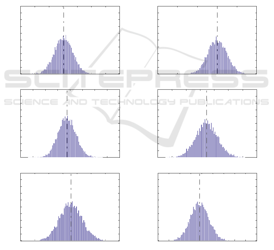
the filter (Elvira,2016). The posterior distributions of
the unknown parameters 𝜃=(𝜏,𝛴
,𝛴
,𝛴
) including
seven joint torques, observation error and noise
generated by the PG algorithm are shown in Fig.1. As
mentioned earlier, 𝛴
,𝛴
,𝛴
are 7×7 diagonal
matrices which diagonal elements are 𝜎1,𝜎2,...,𝜎7.
The same initial settings have been considered for the
PMH algorithm. The proposal density
𝑞(.|𝜃)~𝑁(𝜃,𝐶) where all elements of C, are 10
has been considered. Same as PG algorithm, the
number of the particles in SMC algorithms, were
chosen as N=1000 particles. In practical applications,
the convergence of the algorithms has been checked
to ensure that the samples drawn from the sequential
Markov Chain are sampled from correct target
distributions. The algorithms ran for 10000 steps, and
the first 2500 steps are discarded as burn-in steps.
Table 1 and Table 2 compares the true and estimated
Table 1: True and estimated parameter values for Baxter
manipulator system using PG algorithm.
Table 2: True and estimated parameter values for Baxter
manipulator system using PMH algorithm.
Parameters True values
Estimated
values
Parameters
True
values
Estimated
values
𝜏
1
0.7 0.70007317130
𝜎
1
2e-7 2.6164e-7
𝜏
2
0.6 0.60503887197
𝜎
2
2e-7 1.9921e-7
𝜏
3
1.8 1.79937309232
𝜎
3
2e-7 2.6292e-7
τ
𝜏
4
1 0.99945268679
𝛴
2
𝜎
4
2e-7 2.20990e-7
𝜏
5
0.6 0.59990970609
𝜎
5
2e-7 2.1428e-7
𝜏
6
0.25 0.24996085840
𝜎
6
2e-7 3.5965e-7
𝜏
7
0.085 0.08499487445
𝜎
7
2e-7 2.8616e-7
𝜎
1
2e-7
2.7761 e-7
𝜎
1
2e-7 2.4346e-7
𝜎
2
2e-7
2.8072 e-7
𝜎
2
2e-7
6.6409 e-7
𝜎
3
2e-7
2.9171 e-7
𝜎
3
2e-7
2.6719 e-7
𝛴
1
𝜎
4
2e-7
2.9808 e-7
𝛴
3
𝜎
4
2e-7
5.197 e-7
𝜎
5
2e-7
2.7667 e-7
𝜎
5
2e-7
5.7298 e-7
𝜎
6
2e-7
2.9012 e-7
𝜎
6
2e-7
6.0577 e-7
𝜎
7
2e-7
2.8435 e-7
𝜎
7
2e-7
1.1084 e-7
ICINCO 2023 - 20th International Conference on Informatics in Control, Automation and Robotics
192
parameter values using a PG and PMH algorithms,
respectively. The generated PMH algorithm is not
sensitive to the initial values of parameters.
8 CONCLUSIONS
This paper employs two Particle Markov Chain
Monte Carlo (PMCMC) methods to estimate
unknown parameters of the Baxter robotic
manipulator, including joint torques, noise, and
measurement errors within a nonlinear dynamic
system. Accurate estimates of true state variables are
achieved by estimating state variables within the
State-Space Model. In this study, SMC technique is
employed to estimate the states, and based on these
estimates, the system parameters are further estimated
using both PG and PMH algorithms.
SMC's capability to construct high-dimensional
proposal distributions in each iteration enhances the
reliability of PG and PMH algorithms in estimating
joint torques, noise, and measurement errors. This
contrasts with regular MCMC algorithms, which rely
on lower-dimensional proposal distributions.
Consequently, implementing these methods
enables the precise estimation of unknown robotic
parameters, providing more realistic data for
subsequent investigations.
The results indicate that for the Baxter
manipulator, both PG and PMH algorithms perform
Figure 1: Histogram approximation of posterior densities of parameters τ1, τ2, τ3, τ4, τ5, τ6 based on output of the PG
algorithm.
0.694 0.696 0.698 0.7 0.702 0.704 0.706 0.708
0
50
100
150
200
250
300
350
400
450
500
Estimation of the posterior density
τ
1
Aggregation of samples in each bin
Me a n=0. 70007
0.59 0.595 0.6 0.605 0.61 0.615
0
50
100
150
200
250
300
350
400
450
500
Estimation of the posterior density
τ
2
Aggregation of samples in each bin
Me a n=0.60504
1.7975 1.798 1.7985 1.799 1.7995 1.8 1.8005 1.801 1.8015
0
50
100
150
200
250
300
350
400
450
500
Estimation of the posterior density
τ
3
Aggregation of samples in each bin
Mean=1.7994
0.996 0.997 0.998 0.999 1 1.001 1.002 1.003
0
50
100
150
200
250
300
350
400
450
500
Estimation of the posterior density
τ
4
Aggregation of samples in each bin
Me a n=0.99945
0.5992 0.5994 0.5996 0.5998 0.6 0.6002 0.6004 0.6006
0
50
100
150
200
250
300
350
400
450
500
Estimation of the posterior density
τ
5
Aggregation of samples in each bin
Mean=0.59991
0.2492 0.2494 0.2496 0.2498 0.25 0.2502 0.2504 0.2506 0.2508 0.251
0
50
100
150
200
250
300
350
400
450
500
Estimation of the posterior density
τ
6
Aggregation of samples in each bin
Mean=0.24996
Kinematics Based Joint-Torque Estimation Using Bayesian Particle Filters
193

Figure 2: Histogram approximation of posterior densities of parameters τ
,τ
, τ
,τ
,τ
,τ
based on output of PMH algorithm.
satisfactorily, with PG demonstrating superior
performance owing to its utilization of parameters'
conditional distributions.
REFERENCES
Calderón‐Macías, C., 2000 “Artificial neural networks
for parameter estimation igeophysics”, Geophysical
Prospecting, Vol 48, PP 21-47
Chon,Kh., 1997 “Linear and nonlinear ARMA model
parameter estimation using an artificial neural
network”, IEEE transactions on biomedical, Vol 44, PP
168-174
Van der Merwe, R.,2001, “The square-root unscented
Kalman filter for state and parameter-estimation”,
ICASSP, Vol 6
Wan, E.A., 2000 “The unscented Kalman filter for
nonlinear estimation”, IEEE Adaptive Systems for
Signal Processing, Communications, and Control
Symposium AS-SPCC
0.746 0.748 0.75 0.752 0.754 0.756 0.758 0.76
0
50
100
150
200
250
300
350
400
450
500
Estimation of the posterior density
τ
1
Aggregation of samples in each bin
Me an= 0.75159
0.66 0.665 0.67 0.675 0.68 0.685 0.69
0
50
100
150
200
250
300
350
400
450
500
Estimation of the posterior density
τ
2
Aggregation of samples in each bin
Mean=0.67357
1.728 1.7285 1.729 1.7295 1.73 1.7305 1.731 1.7315 1.732
0
50
100
150
200
250
300
350
400
450
500
Estimation of the posterior density
τ
3
Aggregation of samples in each bin
Mean=1.7296
1.197 1.198 1.199 1.2 1.201 1.202 1.203 1.204 1.205 1.206
0
50
100
150
200
250
300
350
400
450
500
Estimation of the posterior density
τ
4
Aggregation of samples in each bin
Mean=1.2012
0.6994 0.6996 0.6998 0.7 0.7002 0.7004 0.7006 0.7008
0
50
100
150
200
250
300
350
400
450
500
Estimation of the posterior density
τ
5
Aggregation of samples in each bin
Mean=0.70002
0.2795 0.28 0.2805 0.281
0
50
100
150
200
250
300
350
400
450
500
Estimation of the posterior density
τ
6
Aggregation of samples in each bin
Mean=0.28009
ICINCO 2023 - 20th International Conference on Informatics in Control, Automation and Robotics
194

Zargani, J., Necsulescu, R., 2002, “Extended Kalman filter-
based sensor fusion for operational space control of a
robot arm”, IEEE Transactions on Instrumentation and
Measurement, Vol 51, pp 1279-1282
Zarchan, P., 2000 “Fundamentals of Kalman Filtering: A
Practical Approach. American Institute of Aeronautics
and Astronautics” , Incorporated. ISBN 978-1-56347-
455-2
Koblents, E., 2016, “A nonlinear population Monte Carlo
scheme for the Bayesian estimation of parameters of α-
stable distributions” Computational Statistics & Data
Analysis, Vol 95,PP 57-74
Bradley, P., 1992, “A Monte Carlo Approach to Nonnormal
and Nonlinear State-Space Modeling”, Journal of
American Statistical Association, Vol 87
Wenk, C., 1980, “A Multiple Model Adaptive Dual Control
Algorithm for Stochastic Systems with Unknown
Parameters”, IEEE Transactions on Automatic Control,
Vol 25.
D. Bigoni, D., 2012, “Comparison of Classicaland Modern
Uncertainty Quantification Methods for the Calculation
of Critical Speeds in Railway Vehicle Dynamics”. In:
13th mini Conference on Vehicle System Dynamics,
Identification and Anomalies. Budapest,Hungary
Beck, J. V. and Arnold, K. J., 1977, “Parameter Estimation
in Engineering and Science”, Wiley, New York, NY
Cunha, J.B., 2003, “Greenhouse Climate Models: An
Overview”, EFITA conference
Zhang, Z., 1997, “Parameter Estimation Techniques: A
Tutorial with Application to Conic Fitting, Image and
Vision Computing”, Vol 15, pp 59-76
Bigoni, D., 2015, “Uncertainty Quantification with
Applications to Engineering Problems”
Andrieu, C., 2010, “Particle Markov chain Monte Carlo
methods”, Journal of Royal Statistical Society, Vol.72,
PP 269- 342
Nemeth, Ch., 2013, “Sequential Monte Carlo Methods for
State and Parameter Estimation in Abruptly Changing
Environments”, IEEE Transactions on Signal
Processing, Vol 62.
Kantas, N., 2009, “An Overview of Sequential Monte Carlo
Methods for Parameter Estimation in General State-
Space Models”, 15th IFAC Symposium on System
Identification Saint-Malo
Kailath, C. T. Chen, 2010 “Linear Systems”, Springer, PP
94-213.
Wüthrich, M.S., “A new perspective and extension of the
Gaussian Filter” . Int. J. Rob. Res., Vol 35, PP 1731-
1749, https://doi.org/10.1177/0278364916684019.
Grothe, O., 2018, “The Gibbs Sampler with Particle
Efficient Importance Sampling for State-Space
Models”, Institut für Ökonometrie und Statistik,
Universität Köln, Universitätsstr
http://sdk.rethinkrobotics.com/wiki/Arms
Yang C., 2016 “Advanced Technologies in Modern
Robotic Applications”, Springer Science, Chapter 2
Bejczy, A.K, “Robot Arm Dynamic and Control”, National
Aeronautics and Space Administration
Corke, P.I., “A computer tool for simulation and analysis:
the Robotics Toolbox for MATLAB”, CSIRO Division
of Manufacturing Technology
Wackerly, D.D., “ Mathematical Statistics with
Applications”, Thomson, 7th edition
Raiffa, H., 1961, “Applied Statistical Decision Theory.
Division of Research”, Graduate School of Business
Administration, Harvard University
Burkardt, J., “The Truncated Normal Distribution”,
Department of Scientic Computing,Florida State
University
Dahlin, J., “Getting Started with Particle Metropolis-
Hastings for Inference in Nonlinear Dynamical
Models”, University of Newcastle
Elvira, V.“Adapting the Number of Particles in Sequential
Monte Carlo Methods through an Online Scheme for
Convergence Assessment”, IEEE Transaction on
Signal Processing.
Kinematics Based Joint-Torque Estimation Using Bayesian Particle Filters
195
