Visual Counterfactual Explanations Using Semantic Part Locations

Florence B

ottger

, Tim Cech

2 a

, Willy Scheibel

1 b

and J

urgen D

ollner

2 c

University of Potsdam, Digital Engineering Faculty, Hasso Plattner Institute, Germany

University of Potsdam, Digital Engineering Faculty, Germany

Keywords:

Counterfactuals, Explainable Artiﬁcial Intelligence, Convolutional Neural Networks.

Abstract:

As machine learning models are becoming more widespread and see use in high-stake decisions, the ex-

plainability of these decisions is getting more relevant. One approach for explainability are counterfactual

explanations, which are deﬁned as changes to a data point such that it appears as a different class. Their close

connection to the original dataset aids their explainability. However, existing methods of creating counter-

facual explanations often rely on other machine learning models, which adds an additional layer of opacity

to the explanations. We propose additions to an established pipeline for creating visual counterfacual expla-

nations by using an inherently explainable algorithm that does not rely on external models. Using annotated

semantic part locations, we replace parts of the counterfactual creation process. We evaluate the approach

on the CUB-200-2011 dataset. Our approach outperforms the previous results: we improve (1) the average

number of edits by 0.1 edits, (2) the keypoint accuracy of editing within any semantic parts of the image by an

average of at least 7 percentage points, and (3) the keypoint accuracy of editing the same semantic parts by at

least 17 percentage points.

1 INTRODUCTION

In recent years, the impact of machine learning mod-

els has increased in many high-stakes areas, e.g., the

medical ﬁeld (Chen et al., 2021) or autonomous driv-

ing (Schwarting et al., 2018). The topic of ethics in

machine learning for purposes such as bias mitigation

(Wachter et al., 2020) is becoming more prevalent too

(Zhang et al., 2021). However, most models used in

high-stakes decisions are still regarded as black boxes

with little to no inherent means of explaining the mod-

els’ outputs (Castelvecchi, 2016). Given these high

stakes, it is essential that machine learning models

are explainable. In particular, continued use of ma-

chine learning models needs to comply with laws,

e.g., the “right to explanation” from the European

Union’s General Data Protection Regulation (Wachter

et al., 2018).

Solving these problems of explainability is re-

searched within the ﬁeld of Explainable AI (XAI).

While explanations can be generated on models work-

ing with raw data, our focus is on visual explanations.

https://orcid.org/0000-0001-8688-2419

https://orcid.org/0000-0002-7885-9857

https://orcid.org/0000-0002-8981-8583

There exist multiple means of generating explanations

on visual data: some are external to the data, such as

captions (Hendricks et al., 2016) or visual questions

answering, which reveals information by answering

given questions about the decisions (Goyal et al.,

2017; Chen et al., 2020). Others are more closely re-

lated to the data, such as saliency maps, which try to

show the most pertinent parts of an input image (Si-

monyan et al., 2014; Petsiuk et al., 2021). We are fo-

cusing on visual counterfactual explanations, which

are closely related to the input images as we are di-

rectly editing them to generate the explanations.

A Counterfactual Explanation is deﬁned as an edit

of an input image of a given class based on another

image of another class. The initial image and its class

are referred to as the query image and the query class,

while the image that is used for editing and its class

are the distractor image and the distractor class. The

result of this is a counterfactual image, which is based

on the query image while being detected as the dis-

tractor class. For example, a decision of a model to

identify numbers could be explained by displaying

what would need to be changed to instead be detected

as a different number, so a query image showcasing

a “5” should be modiﬁed to instead be detected as

Böttger, F., Cech, T., Scheibel, W. and Döllner, J.

Visual Counterfactual Explanations Using Semantic Part Locations.

DOI: 10.5220/0012179000003598

In Proceedings of the 15th International Joint Conference on Knowledge Discovery, Knowledge Engineering and Knowledge Management (IC3K 2023) - Volume 1: KDIR, pages 63-74

ISBN: 978-989-758-671-2; ISSN: 2184-3228

(a) Query image. (b) Distractor image.

Figure 1: Visual representation of a counterfactual created

by editing a query image with parts of a distractor image

using a vignette overlay. The head of the distractor image is

edited over that of the query image. Note that the vignette

overlay is used to increase visual clarity and is not an exact

representation of the actual counterfactual creation process

and has not been tested in studies.

a distractor class of “6”. By creating a speciﬁc set

of changes from a given data point, the explanation

is intrinsically connected to the data, and therefore it

should be understandable to anyone who understands

the original data. However, this adherence to an orig-

inal data point also limits the scope of possible ex-

planations, as the explanation should not stray too far

from the original, or present impossible or nonsensi-

cal changes. If a counterfactual for the number de-

tection example suggested replacing the entire image,

for example, that would not be a helpful suggestion,

as it would lose all connections to the query image.

A visual representation of a counterfactual can be

seen in Figure 1. A counterfactual has been created

from two images by editing part of the distrator image

over the query image, showing how the query image

subject would need to look different in order to be de-

tected as the distractor class. Note that the vignette

overlay used here is for presentation purposes and is

not an exact representation of the actual process. As

opposed to other methods of explanations, which tend

to be external to the actual data at hand, counterfactu-

als tend to have a much closer connection to the data.

Counterfactual explanations are strongly correlated to

the input; therefore, they are easily understandable.

In particular, a counterfactual explanation can support

causal reasoning, as it displays a change in state and

how it would affect the decision (Pearl, 2000).

One important aspect of counterfactual creation is

comprehensibility: if an edit is incomprehensible to

an observer, for example because it switched a bird’s

head with the legs of another, the explanation would

not be understandable, as it does not present a re-

alistic alternative. Therefore, it is important to en-

courage that the proposed counterfactual explanations

obey this sensibility. Additionally, explanations gen-

erated using external models add an additional layer

of opacity that does not exist when the explanation

itself is more inherently explainable.

In this paper, we expand upon existing approaches

by Goyal et al. (2019) and Vandenhende et al. (2022)

for creating visual counterfactual explanations on the

CUB-200-2011 dataset (Wah et al., 2011) by using

pre-annotated semantic parts data. We outline how we

add an additional loss summand based on annotated

date of semantic parts. We also perform a comparison

of different edits as well as an extensive optimization

of the hyperparameters.

The remainder of this work is structured as fol-

lows. We will ﬁrst go over the related work that we

are building upon. Then we outline our approach,

brieﬂy going over the dataset before explaining the

parts loss, an additional loss term that uses seman-

tic part locations to prefer edits between features con-

taining the same semantic parts. We also add a means

to add tolerance to this process, as well as a way to

simplify the semantic parts in crowded areas. Af-

ter this, we explain the experiment setup, going over

our implementation before elaborating on the relevant

hyperparameters. We also explain the metrics that

we optimize for, then brieﬂy outline our optimiza-

tion algorithm. We perform two experiments, one to

determine viability of different hyperparameters and

one to determine the best values for the hyperparame-

ters that were deemed promising from the ﬁrst exper-

iment, then brieﬂy analyze our approach’s runtime.

After this, we discuss our results, putting them into

perspective and performing comparisons with the pre-

vious work, and evaluate possible threats to validity.

Lastly, we provide our conclusions and detail possible

future work.

2 RELATED WORK

Counterfactual explanations have found widespread

use in explaining machine learning models. Mothilal

et al. (2020) have developed a counterfactual creation

engine for raw information datasets that can create

KDIR 2023 - 15th International Conference on Knowledge Discovery and Information Retrieval

sets of diverse counterfactuals. Gomez et al. (2020)

have created a visual analytics tool to visually repre-

sent counterfactuals to an information dataset. Bor-

eiko et al. (2022) have generated visual counterfac-

tuals by performing detailed edits to change the sub-

ject of the image. As these approaches perform more

complex operations, ensuring semantic context be-

comes a challenge, whereas the approach we are us-

ing performs simpler operations that inherently keep

more of the context intact.

As opposed to more ﬁnely detailed means of coun-

terfactual creation, Goyal et al. (2019) constructed a

visual counterfactual explanation by pasting a subset

of features from the distractor image onto the query

image, resulting in a counterfactual. Because the to-

tal number of possible edits arising from all possible

combinations of features to edit between was too big

to reasonably compute, they proposed a greedy se-

quential search to determine the individual best edits

over multiple edit steps by optimizing a classiﬁcation

loss term.

Vandenhende et al. (2022) expanded upon this

framework by adding a semantic consistency loss

term to the existing greedy sequential search. For this

they used an auxiliary model that determined seman-

tic consistency between spatial cells. They then com-

bined this loss with the classiﬁcation loss and opti-

mized for this combined loss. Additionally, they also

searched over multiple distractor images to ﬁnd the

best edit instead of just one. They optimized for this

by only selecting a smaller number of distractor im-

ages chosen by semantic consistency with the query

image.

Because the semantic consistency approach uti-

lizes an auxiliary model to create its explanation,

someone wishing to fully understand their explana-

tions would also need to understand the auxiliary

model. By adding this additional layer of opacity,

a comprehensive explanation would also need to ex-

plain the auxiliary model. Rudin (2019) argues that

inherently explainable models should be used instead

of black box models when the quality is sufﬁcient.

Our explanation is inherently understandable, as it re-

lies on the annotated parts and matches them between

query and distractor features. As such, no additional

explanation work is needed to fundamentally under-

stand our explanation.

3 APPROACH

Our approach builds upon the previous work done by

Goyal et al. (2019) and Vandenhende et al. (2022).

Ensuring consistency within edits is an important part

of creating understandable edits. For example, an

edit that switches the head of a bird with its wing is

likely to look nonsensical and is therefore ill-suited

as a counterfactual explanation. We can prevent such

edits and therefore improve their accuracy by adding

an additional loss term based on semantic part loca-

tions as well as adding more terms on how said loss is

calculated by implementing a tolerance as well as the

option to simplify semantic parts.

3.1 The Dataset

We use the CUB-200-2011 dataset (Wah et al., 2011)

for our experiments as it has already been used in pre-

vious works by Goyal et al. (2019) and Vandenhende

et al. (2022) in creating visual counterfactuals. It is

also popular among other visual applications of arti-

ﬁcial intelligence, such as the image captioning done

by Hendricks et al. (2016) or the CutMix approach to

training samples proposed by Yun et al. (2019).

The dataset contains 11 788 images of 200 bird

species. It is uniquely suitable to our approach, as

it includes part locations for 15 bird parts, as seen in

Figure 2. We are using these part locations in order to

improve the accuracy of the explanation. According

to the dataset split, 5 794 of the 11 788 images within

the dataset are used for testing, while the others are

used for training.

3.2 Parts Loss

When creating a counterfactual, the basis consists of

an image I of a query class c ∈ C and an image I

a distractor class c

∈ C. The goal is to edit I such

that the result is detected as the class c

. In order to

detect the classes as seen by a given network, a fea-

ture extractor function f : I → R

hw×d

is used, where

h and w are the spatial dimensions of the features

and d the number of channels. A decision network

g : R

hw×d

→ [0, 1]

assigns each feature matrix to a

set of probabilities of the matrix belonging to each

given class.

We perform edits as ﬁrst deﬁned by Goyal et al.

(2019): we permute the features of I

and then edit

only a subset of those features over the features of

I (gating). Consider the permutation matrix P ∈ P,

where P is the set of all hw × hw permutations over

the feature maps, and the gating vector a ∈ {0, 1}

where a

= 1 means that a given feature will be added

to the counterfactual. A counterfactual I

is then ex-

actly deﬁned by P and a:

f (I

∗

) = ( − a) ◦ f (I) + a ◦ P f





. (1)

Visual Counterfactual Explanations Using Semantic Part Locations

Figure 2: The 15 parts labeled within the CUB-200-2011 dataset, as created by Wah et al. (2011).

Table 1: Different types of sub-losses used to calculate total loss. Table is sorted by source date.

Source Loss Formula

Goyal et al. (2019) L

(I, I

) g



( −a)◦ f (I) + a ◦ P f





Vandenhende et al. (2022) L



u(I)

,u(I

)



exp



u(I)

· u (I

)

/τ



∑

∈u(I

)

exp



u(I)

· u (I

)

/τ



Proposed L



r (I)

,r (I

)



max

0≤k<p



r (I)

i,k

· r





j,k



As the dataset we use contains part locations, we

locate the feature within the h × w feature grid that

each part’s spatial location belongs to. We deﬁne

r : I → {0, 1}

hw×p

, (2)

where p is the number of distinct parts in the dataset,

and r(I)

i,k

= 1 if and only if part k is contained within

cell i of the feature representation of I. Our parts loss

is deﬁned in Table 1, where i is the given feature

cell of the query image, and j the cell of the distractor

image. L

is 1 if cell i of the query image and cell j of

the distractor image contain a common class between

them, otherwise it is 0.

Our loss is combined with the loss terms by Goyal

et al. (2019) and Vandenhende et al. (2022) as out-

lined in Table 1 (with u being the auxiliary model and

τ the temperature), leading to the following total loss:



I, I



= logL



I, I



+ λ

· log L



u(I), a





+ λ

· L



r (I) ,a





, (3)

where λ

and λ

are hyperparameters balancing the

individual losses. We keep the use of multiple dis-

tractor images. In the case of n different distractor

images, the semantic class parts for the distractor im-

ages have a combined shape of {0, 1}

nhw×p

3.3 Tolerance for Parts Loss

By default, the semantic class parts for each image

consist of a binary matrix, where a part either exists

within a feature or not. However, the speciﬁc bound-

aries between features are arbitrary with relation to

the image. Therefore, we implement a tolerance sys-

tem to make the result less dependent on said layout.

We deﬁne r

: I → [0,1]

hw×p

similarly to r in

Equation 2. Just as with r, a value of 1 indicates that

a part is present within a feature. However, some-

times parts are close to the boundary between fea-

tures. The previous approach would count them to

be wholly within one feature, even though they are

very close to another. As such, a binary loss is a poor

representation of the reality of the parts.

We take this into account by returning a frac-

tional number within [0, 1] if the part is close to the

given feature. Given an euclidean distance of d be-

tween a class part and a feature cell, the value is

max



0,1 −



, with D being set as the maximum dis-

tance that a cell can have from a part. The unit for

both values is set as the dimension of a cell, so if

e.g. D = 1, the gradient takes effect up to 1 cell away

from the part location. As such, the previously de-

ﬁned function r is equivalent to r

. A comparison of

the approaches can be seen in Figure 3.

We use r

in place of r for the calculation of L

KDIR 2023 - 15th International Conference on Knowledge Discovery and Information Retrieval

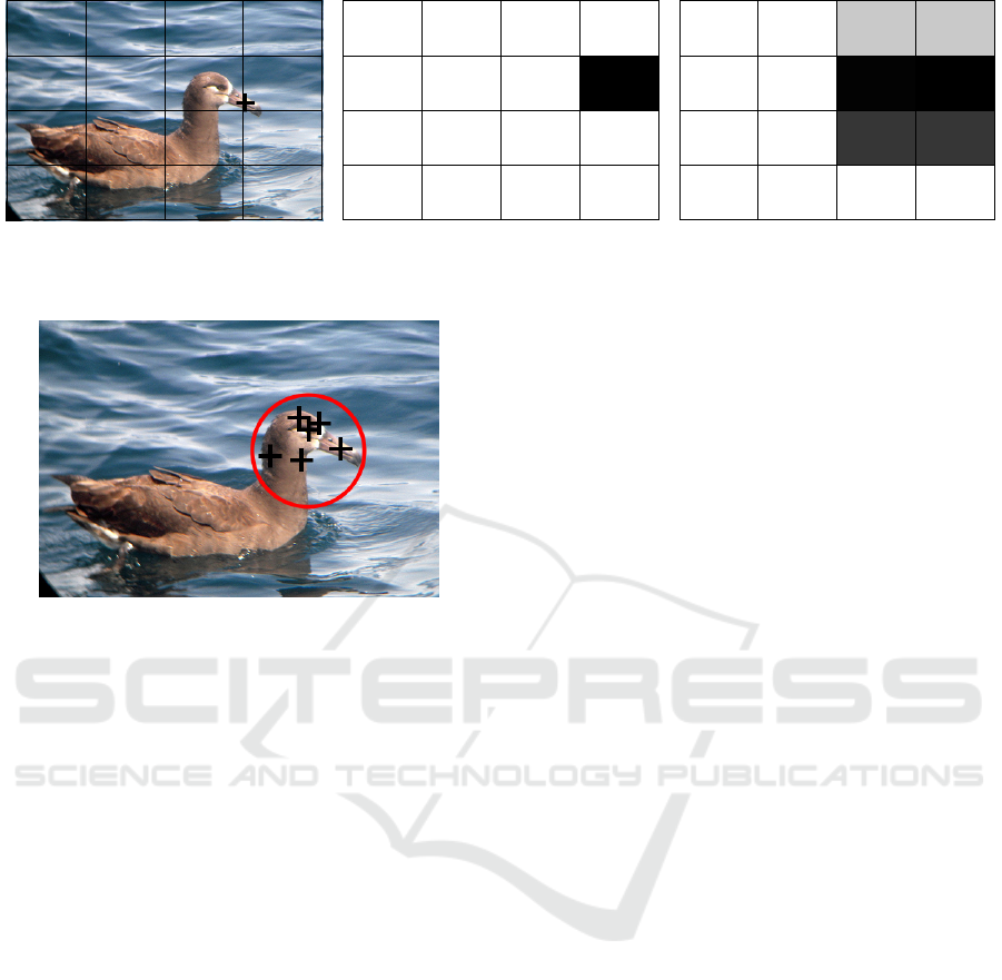
(a) Image with part location.

0.00

1.00

0.00

(b) Matrix for D = 0.

0.00

0.00 0.00

0.21 0.21

0.99

1.00

0.79 0.79

Figure 3: 4 × 4 feature matrices for values of r

for a given part with different tolerances.

Figure 4: Locations of all head parts in an image of a black-

footed albatross from the CUB-200-2011 dataset.

In that case, L



(I)

)



is also no longer a

binary result in {0,1}, but can take any value in [0,1].

3.4 Simplifying Semantic Parts

The annotated part locations may be in different de-

grees of detail based on the speciﬁc dataset and the

purposes said annotation set out to do. For example,

the CUB-200-2011 dataset contains many annotations

for parts within a bird’s head area, as seen in Figure 4.

Such a level of detail is less useful when we are con-

sidering the rougher divisions of the feature grid we

are using. In fact, it might even detract from the result

because the granularity is so much ﬁner than what we

are using. Therefore we are grouping all parts that are

categorized under “head” within Wah et al. (2011) as

the same semantic class.

We use a mapping function m : [0, 1]

hw×p

→

[0,1]

hw×p

, where p

is the new number of parts. Us-

ing a given p × p

permutation matrix M, we calculate

m(R)

i, j

= max

0≤k<p



i,k

· M

k, j



, (4)

where R ∈ [0,1]

hw×p

is a parts matrix. We then use

m(r(I)) and m (r (I

)) in place of r(I) and r (I

), re-

spectively, when calculating L

By performing this simpliﬁcation we are reducing

the total number of semantic parts from the original

15 down to 7 by assigning all classes belonging to the

head—those being the beak, the crown, the forehead,

the eyes, the nape, and the throat—as one “head”

class. Vandenhende et al. (2022) only simpliﬁed the

number of different parts down to 12 by unifying left

and right counterparts of body parts.

4 EXPERIMENT SETUP

We are performing a computational experiment where

we create a counterfactual for each of the 5 794 sam-

ples within the CUB-200-20111 test dataset. The in-

put images within the dataset are of size 224 × 244

pixels, while the feature map has dimensions of 7×7,

meaning that h = w = 7. We use the approach outlined

in section 3 to generate a series of edits by choos-

ing the best edit via L

, as seen in Equation 3, until

the given network predicts the edited features to be-

long to the distractor class. For the sake of creating

counterfactuals between similar semantic classes, we

select the distractor class based on the most similar

class to the query class using a confusion matrix in-

cluded with the dataset. We then randomly select a

given number of distractor images to use for counter-

factual creation. Then we save the counterfactual and

repeat this process for the next one until all of the data

has been processed.

4.1 Implementation

To implement the method outlined above, we are

building upon the Python implementation created by

Vandenhende et al. (2022). Speciﬁcally, we are

adding our additional loss to the sequential greedy

search and expanding upon the program by imple-

menting the necessary hyperparameters as well as

editing the parts map to take tolerance and simpli-

ﬁed parts into account. To compare our results to

Vandenhende et al. (2022), we are using the same

pretrained VGG-16 (Simonyan and Zisserman, 2015)

and ResNet-50 (He et al., 2016) networks that they

Visual Counterfactual Explanations Using Semantic Part Locations

have used.

We perform this experiment using parallelized

computing on four servers (512 GiB RAM each), us-

ing Python version 3.8.13. The code written for this

project as well as additional data are available online

Our results are entirely deterministic, as we are

performing a greedy sequential search. If the hyper-

parameters are identical and the same network is used,

the calculations of the losses for each individual edit

will also be identical. As such the same edits are cho-

sen, and the evaluation is therefore also identical.

4.2 Hyperparameters

For our initial optimization run, we evaluate sev-

eral hyperparameters to determine which ones are the

most promising. As such, we keep the hyperparam-

eter λ

as utilized when weighing L

in the calcula-

tion of the total loss term as ﬁrst proposed by Van-

denhende et al. (2022). In order to still limit the total

number of hyperparameters and yield more substan-

tive results, we are keeping the temperature hyperpa-

rameter τ from Table 1 ﬁxed at the best value deter-

mined by Vandenhende et al. (2022), being τ = 0.1.

We are also adding three additional hyperparame-

ters: λ

from L in Equation 3 is used to determine the

weight of the parts loss L

. D is be used to balance

the tolerance for the semantic class loss using r

, as

outlined in subsection 3.3. Lastly, we use a binary hy-

perparameter S ∈ {True, False} to determine whether

we further simplify the semantic parts from 12 parts

to 7. We set 0 ≤ λ

≤ 2, 0 ≤ λ

≤ 10, 0 ≤ D ≤ 3 and

S ∈ {True, False} as the optimization ranges for the

hyperparameters.

4.3 Optimization Metrics

We use the evaluation metrics initially used by Goyal

et al. (2019) and Vandenhende et al. (2022), those be-

ing the average number of edits as well as the keypoint

(KP) metrics. Let m be the size of the dataset we are

editing over, and E

∈ N,0 ≤ k < m the number of ed-

its on the k-th iteration. Then the average amount of

edits E is

E =

∑

m−1

k=0

. (5)

For the keypoint metrics, consider a single given

edit e = (i, j) ∈ (N,N) , 0 ≤ i, j < hw consisting of a

pair of a query cell i from I and a distractor cell j

from I

to edit. Then the Near-KP metric of that edit

: N

hw×hw

→ [0,1] is deﬁned as the average num-

https://doi.org/10.5281/zenodo.8056313

Table 2: Spearman correlation between different metrics

over initial testing using VGG-16 and 400 iterations. Note

that for clarity, −E is used in place of E as we wish to min-

imize E while maximizing the KP values.

−E KP

S,N

S,S

A,N

A,S

−E 1 −0.44 −0.60 0.01 −0.26

S,N

−0.44 1 0.89 0.86 0.91

S,S

−0.60 0.89 1 0.67 0.90

A,N

0.01 0.86 0.67 1 0.89

A,S

−0.26 0.91 0.90 0.89 1

ber of these cells which contain at least one semantic

part within them:

(i, j) =

p−1

[

k=0

r(I)

i,k

= 1

p−1

[

k=0





j,k

= 1

. (6)

The Same-KP metric KP

: N

hw×hw

→ {0, 1} is

deﬁned as being 1 if the edit cells share a common

semantic part between them and 0 otherwise:

(i, j) =

p−1

[

k=0

r(I)

i,k

= r





j,k

= 1

. (7)

For both of these individual edit metrics, we de-

ﬁne both a variant deﬁned as the total average of the

given metric for all edits across each iteration and a

variant deﬁned as the average of only the single ﬁrst

edit across each iteration. This results in ﬁve total

metrics: the average number of edits E, the Near-KP

over a single edit KP

S,N

, the Near-KP over all edits

A,N

, the Same-KP over a single edit KP

S,S

and the

Same-KP over all edits KP

A,S

We speciﬁcally focus on two metrics for the op-

timization: the average number of edits E and the

Same-KP over all edits KP

A,S

. These metrics were

chosen as early tests have shown that the different

keypoint metrics largely correlate with one another,

while edits show little or even opposed correlation

with the keypoint metrics, as seen in Table 2. Note

that we are using −E instead of E in the table, as we

wish to minimize E while maximizing the KP values.

As E is inversely correlated with all of the other

metrics that we considered, it was chosen as one of

our main metrics. From the KP metrics, we choose

the Same-KP over all edits KP

A,S

. This metric is the

strictest, as early tests have shown that KP

A,S

yields

the lowest average out of all keypoint metrics. Fol-

lowing, we refer to the KP

A,S

metric as KP.

KDIR 2023 - 15th International Conference on Knowledge Discovery and Information Retrieval

Figure 5: Scatter plot of all 400 optimization iterations from

initial testing using VGG-16. The Pareto front is high-

lighted in red.

4.4 Optimization Algorithm

We use the optimization framework Optuna (Ak-

iba et al., 2019) in order to optimize the given hy-

perparameters. This framework lets the user have

freedom in constructing the search space (deﬁne-by-

run principle). We slot the existing structure that

we expanded from the work by Vandenhende et al.

(2022) into an optimization function without requir-

ing drastic changes or forgoing the existing function-

ality of externally-deﬁned hyperparameters. We then

use Optuna to optimize the existing functions, utiliz-

ing a tree-structured Parzen estimator (Bergstra et al.,

2011). We chose this estimator due to its good perfor-

mance even for multivariate optimization.

5 EXPERIMENTS

In order to showcase our results, we perform two ex-

periments. Experiment 1 is performed to analyze the

quality of our four selected hyperparameters by con-

sidering their correlation with our two metrics. From

among those we then select the hyperparameters that

have a positive correlation with at least one of the

metrics. Experiment 2 is performed with just these

hyperparameters with the goal of determining the to-

tal quality of our results. We are also comparing our

results with those set by Goyal et al. (2019) and Van-

denhende et al. (2022).

5.1 Experiment 1

We begin by performing an optimization using VGG-

16 and all four hyperparameters (λ

, λ

, D, and S)

over 400 iterations to determine the viability of each

of the hyperparameters. A scatter plot of the results

from this test can be seen in Figure 5. In order to

Table 3: Spearman correlation and related p-values between

the hyperparameters and the optimization metrics over the

ﬁrst experiment using VGG-16.

p(r

) r

p(r

)

-0.03 56% 0.91 < 0.1%

0.47 < 0.1% 0.19 < 0.1%

D -0.68 < 0.1% -0.35 < 0.1%

S -0.23 < 0.1% 0.08 10.1%

Table 4: Spearman correlation and related p-values between

the hyperparameters and the optimization metrics over the

second experiment using VGG-16.

p(r

) r

p(r

)

0.77 < 0.1% 0.82 < 0.1%

D -0.57 < 0.1% -0.48 < 0.1%

determine the impact of each hyperparameter, we de-

termine the Spearman correlation (Spearman, 1904)

of each hyperparameter on each of the optimization

metrics. The Spearman correlation is deﬁned as the

correlation between the ranks of a set of values, mean-

ing it measures monotony. The reason we utilize the

Spearman correlation is that we mainly wish to deter-

mine the hyperparamters’ impact on the rank of the

values so we can determine their general impact. We

also record the corresponding p-values for the null

hypothesis that the hyperparameter has no correlation

with the metric.

As can be seen from Table 3, λ

has a very slight

negative correlation on KP, while also having a very

direct correlation with a higher E. λ

, meanwhile,

has a rather clear correlation with a higher KP, while

slightly increasing E. D has a negative correlation

on KP, while correlating with fewer edits E. Lastly,

S appears to have negative correlation on KP while

appearing to have little correlation to E.

Given these correlation values, we can determine

that λ

and D each positively correlate with one of our

metrics: while λ

correlates with better KP, D corre-

lates with fewer edits. The other two metrics which

we tested in these experiments, λ

and S do not dis-

play a positive correlation with either of our metrics.

Therefore, Experiment 2 will be performed using the

hyperparameters λ

and D with both the VGG-16 and

ResNet-50 models.

5.2 Experiment 2

For optimizing the results using only the hyperparam-

eters λ

and D, we begin by queuing up optimization

trials for the extreme values of λ

= 0, D = 0 and

= 10, D = 0. Early tests have shown that these val-

Visual Counterfactual Explanations Using Semantic Part Locations

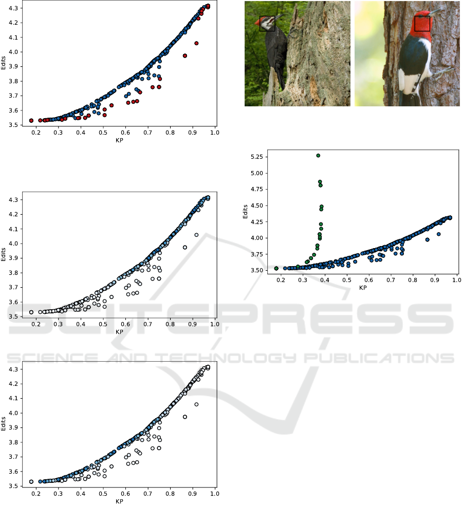
Figure 6: Scatter plot of all 400 iterations from the second

experiment using VGG-16. The Pareto front is highlighted

in red.

(a) λ

(b) D.

Figure 7: Scatter plot of all 400 iterations of the second

experiment using VGG-16. The saturation of the data points

indicates the value of a given hyperparameter, with more

saturation corresponding to higher values.

ues provide extreme values for the results, and choos-

ing them for the initial optimization trials sets a range

for the optimization, as well as providing promising

initial values. A scatter plot of the 400 optimization

iterations for this experiment using VGG can be seen

(a) Query image. (b) Distractor image.

Figure 8: Features to be edited from a query-distractor pair.

Figure 9: Scatter plot of 400 iterations from the second ex-

periment using VGG-16 (blue) and scatter plot of 18 grid

search samples from Vandenhende et al. (2022) (green).

in Figure 6. When visualizing the hyperparameters

via the saturation of the data points in Figure 7, we

can see a tradeoff between λ

correlating to good KP

but poor E, while D correlates with worse KP but bet-

ter E. This is also reﬂected in the Spearman correla-

tion in Table 4, which shows a strong correlation with

and a good KP but many edits, and the opposite

for D.

In order to showcase visual results, a choice of a

speciﬁc hyperparameter pair is necessary. We opted

to choose λ

= 0.51, D = 0.09 from the pareto front,

which yields 3.65 average edits and an average KP of

61.1%. For these hyperparameters, we showcase the

ﬁrst edit in Figure 8. We can see that the ﬁrst edit is

identiﬁed to be between the heads of the birds.

Figure 9 shows a comparison of our work to that

of Vandenhende et al. (2022). We note that when

they performed a grid search on their hyperparame-

ters (those being λ

and τ), it was without some of

the other improvements they have added, such as only

considering one distractor image instead of choosing

out of multiple ones. For the sake of a fair compar-

ison, we repeat their grid search with the addition of

their improvements.

Our results consistently outperform those of Van-

denhende et al. (2022) along both metrics. The data

KDIR 2023 - 15th International Conference on Knowledge Discovery and Information Retrieval

Table 5: Comparison of all metrics between Goyal et al. (2019), Vandenhende et al. (2022), and our implementation on a

VGG-16 network. KP are given in %. We are listing both a balanced set of hyperparameters with λ

= 0.51, D = 0.09 as

well as a KP-optimizing set of hyperparameters at λ

= 10, D = 0. The best results for each metric are bolded.

E KP

S,N

S,S

A,N

A,S

Goyal et al. (2019) 5.5 67.8 17.2 54.6 8.3

Goyal et al. (2019) (Multiple Distractors) 3.5 75.3 24.2 70.4 17.8

Vandenhende et al. (2022) 3.8 78.1 41.0 71.9 36.5

Proposed 3.7 85.4 58.7 83.7 61.1

Proposed (KP Optimized) 4.3 100.0 100.0 97.7 96.9

point with the lowest KP and edits is the data point

where the respective weight hyperparameter λ

or λ

is 0, meaning that only the classiﬁcation loss L

considered. This point is the equivalent to the initial

approach by Goyal et al. (2019), though with the ad-

ditional features Vandenhende et al. (2022). A full

overview of the results for the edits and all KP met-

rics can be seen in Table 5. In addition to the results

from the related work, we have also added results for

the Goyal et al. (2019) approach of only using L

(i.e.

= λ

= 0) with later additions such as multiple dis-

tractor images, as well as our balanced set of hyper-

parameters with λ

= 0.51, D = 0.09 and a set with

= 10, D = 0 which optimizes the KP metrics.

Notably, when optimizing for KP metrics, we can

see that we reach exactly 100% on the single-edit

evaluations. This means that the ﬁrst edit is always

between two features that share a common part. How-

ever, this also leads to the highest number of edits

out of any of the multi-distractor approaches. On

the other hand, using only L

in the loss calculation

while using multiple distractors yields the fewest ed-

its, but it also features the worst KP metrics out of

the multi-distractor approaches. Both the approach

by Vandenhende et al. (2022) and our balanced one

have results in between these extremes, with our bal-

anced approach consistently outperforming theirs in

each metric. While edits are only slightly improved

by 0.1 edits, the KP values are improved by at least

7 percentage points at their lowest and up to 24 per-

centage points at their highest.

5.3 Runtime Performance

We perform a runtime analysis using the conditions

of Experiment 1, i.e. 400 optimization iterations us-

ing all hyperparameters. Using these conditions, we

achieve a maximum runtime of 6449.5 seconds, a

minimum runtime of 4239.7 seconds, and an average

runtime of 5010.5 seconds. The average time per edit

is 0.255 seconds. Note that as this is an optimization,

it is to be expected that the results improve during it,

and as such, runtime also improves.

This can be seen when comparing the correlation

between the number of edits and the total runtime of

each optimization iteration. Given that we analyze

how accurate the average runtime is, we will perform

a Pearson correlation analysis (Pearson, 1896) in ad-

dition to a Spearman one. Because Pearson correla-

tion indicates the correlation of the raw values instead

of the ranks as Spearman does, a high Pearson corre-

lation indicates a linear relationship between the num-

ber of edits and the runtime, meaning that it strongly

indicates whether the average time per edit is accurate

to most edits. The values have a Pearson correlation

of ρ = 0.995, a Pearson p-value of < 0.1%, a Spear-

man correlation of r = 0.992, and a Spearman p-value

of < 0.1%. This shows that the runtime of a given edit

is largely similar among different executions, so the

true measure for the runtime is how many total edits

are occurring.

6 DISCUSSION

Our approach outperforms existing counterfactual

creation approaches within the KP and edits metrics.

By adding the parts loss L

and therefore speciﬁ-

cally encouraging edits that will optimize the KP met-

rics, we are able to especially achieve higher KP met-

rics. There exist especially large improvements on the

Same-KP metric, indicating that our approach edits

between the same semantic parts more frequently than

previous work. This becomes clear when consider-

ing the ratio of Same-KP to Near-KP, which indicates

how many edits that concerned a semantic part also

edited between the same semantic parts. In the ap-

proach by Vandenhende et al. (2022), when consider-

ing only the ﬁrst edit, this ratio is 52.5%, and over all

edits it drops to 50.8%. In our approach, meanwhile,

on the ﬁrst edit, the ratio is 68.8%, and this ratio actu-

ally rises to 73.0% over all edits. This shows that the

Same-KP metrics rose comparatively higher than the

Near-KP metrics.

However, we note that these metrics are still only

approximations of the actual goal of the ﬁeld of XAI,

Visual Counterfactual Explanations Using Semantic Part Locations

that being creating explanations that are understand-

able to humans. While better performance in these

metrics has correlated with better results in the user

study performed by Vandenhende et al. (2022), this

does not necessarily apply in every circumstance.

Choice of metrics in general is not a settled topic

(Vilone and Longo, 2021), with Rosenfeld (2021)

proposing a general set of metrics that generally lead

to simpler and more inherently explainable models

being preferred. As such, if the user-based metrics

for our approach are poor in comparison to the greater

performance of the heuristics-based metrics, a differ-

ent choice of metrics may better represent the impact

on the users.

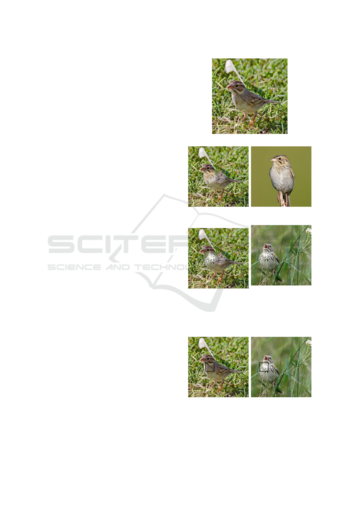
Goyal et al. (2019) presented some of their coun-

terfactual explanations by merging the edited features

over the query image via vignette masks. A display

of this approach can be seen in Figure 10. This ap-

proach displays a smoother approximation of edits

and is likely to be more pleasant viewing than a more

discrete pasting of a feature rectangle would be. How-

ever, while it does make for a comparatively prettier

representation, it is not quite accurate to the process of

counterfactual approximation. Within the actual pro-

cess, the entirety of the feature is edited.

Examples such as Figure 10 show that while our

approach performs well within the metrics, the ap-

proach by Vandenhende et al. (2022) tends to pro-

duce smoother transitions. For instance, while our

approach edits the chest area in such a way that pro-

duces visible tears, Vandenhende et al. (2022) manage

to edit the chest area in such a way that the transi-

tion appears seamless. However, merged images such

as these have not actually been used within the user

studies tracking understandability of the explanations

by Goyal et al. (2019) and Vandenhende et al. (2022).

Instead, the features to be edited were represented us-

ing bounding boxes as seen in Figure 11. While our

merged images do not look as seamless as those in

the semantic consistency approach, the bounding box

representation in this ﬁgure still shows an edit be-

tween the breasts of the birds.

Internal threats to validity can occur from our

heavy reliance on the parts annotation, which is a

comparatively less-utilized aspect of the CUB-200-

2011 dataset. Errors within said annotations would

greatly inﬂuence the results.

Regarding external threats, it is impossible to uti-

lize the parts loss on datasets without semantic part

locations. The speciﬁc hyperparameter values for the

tolerance distance D are also only valid within the

context of the speciﬁc parts within the CUB-200-2011

dataset that they were optimized for, as well as rely-

ing on consistent feature grid dimensions to remain

(a) Query image.

(b) Merged (Vandenhende

et al., 2022).

denhende et al., 2022).

(d) Merged (Proposed).

(e) Distractor image (Pro-

posed).

Figure 10: Merged images of the query image and counter-

factual features using a vignette mask as well as the distrac-

tor images for the second edit, comparing our approach and

the one by Vandenhende et al. (2022).

(a) Query image. (b) Distractor image.

Figure 11: Features to be edited from a query-distractor pair

for our approach on the second edit.

KDIR 2023 - 15th International Conference on Knowledge Discovery and Information Retrieval

accurate. Changing the dataset or the feature grid

dimensions would require optimizing these hyperpa-

rameters once more. In comparison, the approach by

Vandenhende et al. (2022) is more generically appli-

cable, as semantic consistency is transferable between

models and does not require any additional training or

optimization once the auxiliary model has been ini-

tially trained. As such, our speciﬁc results are only

applicable to this dataset and only generalizable to a

speciﬁc subset of datasets. The fact that an improve-

ment over the state of the art exists, even if limited

to a speciﬁc dataset, may encourage the creation of

similar annotations on further datasets.

Additionally, within the ﬁrst experiment, we only

determine correlation, which is not causation. While

we perform multiple experiments to conﬁrm our hy-

potheses and reach very low p-values within them, it

is nonetheless not a guaranteed indication of causa-

tion. Because we determine the Spearman correlation

on data that is gained from optimization, it is possible

that the optimization itself acts as a confounder, lead-

ing to uncorrelated hyperparameters to be be seen as

correlated (Pearl, 2000). This is an especially high

risk in the case of the hyperparameter S due to its

binary state. Assuming that it is uncorrelated to be-

gin with, random sampling may still create the im-

pression that it is correlated in some way. Therefore

the optimization algorithm might prefer that value for

S in further tests, leading to a potentially inaccurate

view of the actual level of correlation. However, this

can only create the impression of a correlation where

there is none, and given that S and λ

showed a neg-

ative correlation, they are either actually negatively

correlated or not correlated. Either way, they would

not be viable candidates. The positive correlation of

and D in respect to one of the metrics each has been

observed over multiple optimization runs for both the

ﬁrst experiment and additionally for both the VGG-

16 and ResNet-50 networks within the second exper-

iment. Therefore, while it is impossible to rule out, it

is unlikely that λ

or D are not actually correlated to

the metrics.

7 CONCLUSIONS & FUTURE

WORK

In this work we have presented an approach for cre-

ating visual counterfactual explanations based upon

a new parts loss term L

. This loss term takes into

account the accuracy of an edit with regards to the se-

mantic parts, controlled by a hyperparameter λ

. We

also created hyperparameters to add to this loss by

adding a distance tolerance D to account for the arbi-

trary nature of the bounds between features, as well

as an option S to simplify the semantic parts within

the high-density area of the head. Using an in-depth

optimization process, we then determined the perfor-

mance of the new hyperparameters. This is opposed

to the semantic loss term L

originally introduced by

Vandenhende et al. (2022) which used an external net-

work to measure semantic similarity.

Our evaluation determined that the hyperparam-

eter λ

controlling semantic loss L

has little cor-

relation with the keypoint metrics, and strong nega-

tive correlation with the number of edits. We also

determined similar results for the simpliﬁcation op-

tion S. As such we focused on experiments using

only the hyperparameters λ

and D. By optimiz-

ing these two hyperparameters we could ﬁnd conﬁg-

urations that outperform the standard set by Vanden-

hende et al. (2022). In particular we improve upon

their work by an average of 0.1 edits and at least 7

percentage points in the keypoint metrics when con-

sidering the keypoints generally being part of the bird

and at least 17 percentage points when considering if

the edits share a semantic part.

We have created an explanation algorithm that is

inherently explainable which outperforms the previ-

ous work while not relying on an external model. By

using metadata such as semantic part locations, this

approach could be expanded to other data sets.

In the future, we plan to perform user studies to

determine whether the improved metrics of our ap-

proach lead to more understandable explanations. We

also invite other researchers to investigate if similar

types of metadata from other datasets could be used

to improve the performance of this or other explana-

tion approaches on those datasets.

ACKNOWLEDGEMENTS

We thank the anonymous reviewers for their valu-

able feedback. This work was partially funded by

the German Federal Ministry for Education and Re-

search (BMBF) through grant 01IS22062 (“AI re-

search group FFS-AI”).

REFERENCES

Akiba, T., Sano, S., Yanase, T., Ohta, T., and Koyama, M.

(2019). Optuna: A next-generation hyperparameter

optimization framework. In Proc. 25th ACM SIGKDD

International Conference on Knowledge Discovery

and Data Mining, KDD ’19, pages 2623–2631. ACM.

Bergstra, J., Bardenet, R., Bengio, Y., and K

egl, B.

(2011). Algorithms for hyper-parameter optimiza-

Visual Counterfactual Explanations Using Semantic Part Locations

tion. In Proc. Neural Information Processing Systems,

NeurIPS ’11. Curran Associates, Inc.

Boreiko, V., Augustin, M., Croce, F., Berens, P., and Hein,

M. (2022). Sparse visual counterfactual explanations

in image space. In Proc. DAGM German Conference

on Pattern Recognition, GCPR ’22, pages 133–148.

Springer International Publishing.

Castelvecchi, D. (2016). Can we open the black box of AI?

Nature News, 538(7623):20–23.

Chen, I. Y., Pierson, E., Rose, S., Joshi, S., Ferryman, K.,

and Ghassemi, M. (2021). Ethical machine learning

in healthcare. Annual Review of Biomedical Data Sci-

ence, 4:123–144.

Chen, L., Yan, X., Xiao, J., Zhang, H., Pu, S., and Zhuang,

Y. (2020). Counterfactual samples synthesizing for

robust visual question answering. In Proc. IEEE/CVF

Conference on Computer Vision and Pattern Recogni-

tion, pages 10797–10806. IEEE.

Gomez, O., Holter, S., Yuan, J., and Bertini, E. (2020).

ViCE: Visual counterfactual explanations for machine

learning models. In Proc. 25th International Con-

ference on Intelligent User Interfaces, IUI ’20, pages

531–535. ACM.

Goyal, Y., Khot, T., Summers-Stay, D., Batra, D., and

Parikh, D. (2017). Making the V in VQA matter: Ele-

vating the role of image understanding in visual ques-

tion answering. In Proc. IEEE/CVF Conference on

Computer Vision and Pattern Recognition, CVPR ’17,

pages 6325–6334. IEEE.

Goyal, Y., Wu, Z., Ernst, J., Batra, D., Parikh, D., and

Lee, S. (2019). Counterfactual visual explanations.

In Proc. 36th International Conference on Machine

Learning, PMLR ’19, pages 2376–2384. PMLR.

He, K., Zhang, X., Ren, S., and Sun, J. (2016). Deep

residual learning for image recognition. In Proc. Con-

ference on Computer Vision and Pattern Recognition,

CVPR ’16, pages 770–778. IEEE.

Hendricks, L. A., Akata, Z., Rohrbach, M., Donahue, J.,

Schiele, B., and Darrell, T. (2016). Generating visual

explanations. In Proc. European Conference on Com-

puter Vision, ECCV ’16, pages 3–19.

Mothilal, R. K., Sharma, A., and Tan, C. (2020). Explaining

machine learning classiﬁers through diverse counter-

factual explanations. In Proc. Conference on Fairness,

Accountability, and Transparency, FAT* ’20, pages

607–617. ACM.

Pearl, J. (2000). Causality: Models, Reasoning and Infer-

ence. Cambridge University Press.

Pearson, K. (1896). VII. Mathematical contributions to the

theory of evolution.—III. Regression, heredity, and

panmixia. Philosophical Transactions of the Royal

Society of London. Series A, containing papers of a

mathematical or physical character, 187:253–318.

Petsiuk, V., Jain, R., Manjunatha, V., Morariu, V. I., Mehra,

A., Ordonez, V., and Saenko, K. (2021). Black-box

explanation of object detectors via saliency maps. In

Proc. IEEE/CVF Conference on Computer Vision and

Pattern Recognition, CVPR ’21, pages 11438–11447.

IEEE.

Rosenfeld, A. (2021). Better metrics for evaluating ex-

plainable artiﬁcial intelligence. In Proc. 20th Interna-

tional Conference on Autonomous Agents and Multia-

gent Systems, AAMAS ’21, pages 45–50. IFAAMAS.

Rudin, C. (2019). Stop explaining black box machine learn-

ing models for high stakes decisions and use inter-

pretable models instead. Nature Machine Intelligence,

1(5):206–215.

Schwarting, W., Alonso-Mora, J., and Rus, D. (2018). Plan-

ning and decision-making for autonomous vehicles.

Annual Review of Control, Robotics, and Autonomous

Systems, 1:187–210.

Simonyan, K., Vedaldi, A., and Zisserman, A. (2014).

Deep inside convolutional networks: Visualising im-

age classiﬁcation models and saliency maps. In Proc.

2nd International Conference on Learning Represen-

tations – Workshops Track, ICLR ’14.

Simonyan, K. and Zisserman, A. (2015). Very deep convo-

lutional networks for large-scale image recognition. In

Proc. 3rd International Conference on Learning Rep-

resentations, ICLR ’15, pages 1–14. Computational

and Biological Learning Society.

Spearman, C. E. (1904). The proof and measurement of

association between two things. American Journal of

Psychology, 15(1):72–101.

Vandenhende, S., Mahajan, D., Radenovic, F., and Ghadi-

yaram, D. (2022). Making heads or tails: Towards se-

mantically consistent visual counterfactuals. In Proc.

European Conference on Computer Vision, ECCV

’22, pages 261–279. Springer Nature Switzerland.

Vilone, G. and Longo, L. (2021). Notions of explainability

and evaluation approaches for explainable artiﬁcial in-

telligence. Information Fusion, 76:89–106.

Wachter, S., Mittelstadt, B., and Russell, C. (2018). Coun-

terfactual explanations without opening the black box:

Automated decisions and the GDPR. Harvard Journal

of Law & Technology, 31(2):841–887.

Wachter, S., Mittelstadt, B., and Russell, C. (2020). Bias

preservation in machine learning: The legality of fair-

ness metrics under EU non-discrimination law. West

Virginia Law Review, 123(3):735–790.

Wah, C., Branson, S., Welinder, P., Perona, P., and Be-

longie, S. (2011). The Caltech-UCSD Birds-200-2011

dataset. Technical Report CNS-TR-2011-001, Cali-

fornia Institute of Technology.

Yun, S., Han, D., Oh, S. J., Chun, S., Choe, J., and Yoo,

Y. (2019). CutMix: Regularization strategy to train

strong classiﬁers with localizable features. In Proc.

IEEE/CVF International Conference on Computer Vi-

sion, (ICCV ’19, pages 6022–6031. IEEE.

Zhang, B., Anderljung, M., Kahn, L., Dreksler, N.,

Horowitz, M. C., and Dafoe, A. (2021). Ethics and

governance of artiﬁcial intelligence: Evidence from

a survey of machine learning researchers. Journal of

Artiﬁcial Intelligence Research, 71:591–666.

KDIR 2023 - 15th International Conference on Knowledge Discovery and Information Retrieval