Locally Convex Neural Lyapunov Functions and Region of Attraction

Maximization for Stability of Nonlinear Systems

Lucas Hugo

, Philippe Feyel

and David Saussi´e

Robotics and Autonomous Systems Laboratory, Polytechnique Montr´eal, Montr´eal, Qu´ebec H3T1J4, Canada

Safran Electronics & Defense Canada, Montr´eal, Canada

Keywords:

Lyapunov Functions, Stability, Neural Network Optimization, Convexity, Region of Attraction.

Abstract:

The Lyapunov principle involves to ﬁnd a positive Lyapunov function wi th a local minimum at the equilibrium

point, whose time derivative is negative with a local maximum at that point. As a validation, it is usual to

check the sign of the Hessian eigenvalues which can be complex: it requires to know a formal expression of

the system dynamics, and especially a differentiable one. In order to circumvent this, we propose in this paper

a scheme allowing to validate these functions without computing the Hessian. Two methods are proposed

to force the convexity of the function near the equilibrium; one uses a neural single network to model the

Lyapunov function, the other uses an additional one to approximate its time derivative. The training process

is designed to maximize the region of attraction of the locally convex neural Lyapunov function trained. The

use of examples allows us to validate t he efﬁciency of this approach, by comparing it with the Hessian-based

approach.

1 INTRODUCTION

Lyapunov theory is a commonly used tool in control

theory to analyse stability of dynamical systems. A

Lyapunov function can be used to de te rmine the equi-

librium stability of nonlinear systems, as well as to

estimate the Region of Attraction (RoA) or establish

a stabilizing c ontrol (Mawhin, 2005; Khalil, 2001).

This type of potential function keeps track of the en-

ergy dissipated by a system. In addition to modelling

physical en ergy, a Lyapunov function can also rep-

resent abstract quantities provided it fulﬁlls the fol-

lowing p roperties: (1) it must be a positive deﬁnite

function locally, (2) it must have continuous partial

derivatives, and (3) its time derivative a long any state

trajectory must be negative semi- deﬁnite.

There are many ways of ﬁnding a Lyapunov func-

tion in the literature, each one of th em with its draw-

backs and a dvantages (Giesl and Hafstein, 2015), but

recently optimization methods based on neural net-

works training have increased signiﬁcantly. Indeed,

the ability of neural networks to represent a func-

tion has been well established since the ea rly 90s

(Cybenko, 1989; Hornik et al., 1989; Hornik , 1991;

Liang and Srikant, 2017). Neural approximations

https://orcid.org/0000-0002-4228-1109

were ﬁrst used to determine Lyapunov candidates for

nonlinear autonomous systems in (Prokhorov, 1994)

and various metho ds have since been proposed to

guide network training.

(Petridis and Petridis, 2006) develop an Hessian-

based approa c h to ensure a strict validation of

Lyapunov properties near an equilibrium and

(Bocquillon et al., 2022) extend it to prove asymp-

totic, exponential or ISS stability of continuou s or

discrete time systems usin g a genetic algorithm. The

network structure in these works is restricted to a

single hidden layer network, and they require to know

a differentiable expression of the system d ynamics.

(Richards et al., 2018) propose a training framework

based on an iterative gradient-d escent to estimate the

largest possible RoA fo r general nonlinear dynamica l

systems with structural properties on activation

functions and weighting matr ic e s. To completely

avoid structural limitations o n the trained network,

(Chang et al., 2020) repea ts multiple gradient-based

optimization pro blems to identify states that vio-

late Lya punov conditions and (Ga by et al., 2022)

propose a versatile neural ne twork architecture

called Lyapunov-Net that ensure positive deﬁn iteness

of the Lyapunov candida te while simplifying the

optimization problem formulation. Nevertheless a

concession is made in terms of training efﬁciency

Hugo, L., Feyel, P. and Saussié, D.

Locally Convex Neural Lyapunov Functions and Region of Attraction Maximization for Stability of Nonlinear Systems.

DOI: 10.5220/0012180300003543

In Proceedings of the 20th International Conference on Informatics in Control, Automation and Robotics (ICINCO 2023) - Volume 1, pages 29-36

ISBN: 978-989-758-670-5; ISSN: 2184-2809

as the c ost functions used needs to converge to 0 so

that the Lyapunov candidate obtained strictly validate

Lyapunov properties, especially near the equilibrium.

To circumvent this issue (Chang and Gao, 2021)

introdu ce the c oncept of Almost Lyapunov functions,

theoretically relevant but difﬁcult to validate in

practice.

To provide a tool with the sam e validity guarantee

as the Hessian-b ased approach, but app lica ble to gen-

eral non-linear systems that are not necessarily dif-

ferentiable, we propose two methods to train locally

convex neural Lyapunov functions with the ﬂexibil-

ity of an optimization-based approach. The fra me-

work is designed so tha t time der ivative function local

concavity is guided by the cost function while loca l

convexity of the Lyapunov function is stru cturally en-

forced, allowing a great liberty of network structure,

while maximizing the RoA.

This pa per is structured as follows. Preliminaries

related to Lyapunov theory are introduc e d in section

2. In section 3, we present the two methods to train

locally convex neural Lyapunov function, one uses a

single network to model the Lyapunov function, the

other uses an additional network to approx imate its

time derivative. Finally, we illustrate in section 4 the

efﬁciency of our approaches with examples, by com-

paring it with the Hessian-based approach.

2 PRELIMINARIES

Notations and deﬁnitions used in this paper are intro-

duced in this section. Let R denote the set of real

numbers, ||.|| denote the eu clidean norm on R

the

disjoint union between sets, and X ⊂ R

, a set c on-

taining x = 0.

This pa per deals with following autonom ous sys-

tems:

x = f(x) (1)

where f : X −→ R

is a locally Lipschitz map with

at least one equilibrium point x

, that is f(x

) = 0.

Throu ghout this pap er, the equilibrium point is com-

monly set at the origin, x

= 0 without loss of gener-

ality.

Theorem 2.1 (Lyapunov Theory). (Khalil, 2001)

Let V : X −→R be a continuously differentiable func-

tion,

V (x

) = 0 and V (x) > 0 in X −{x

} (2)

V (x) ≤ 0 in X (3)

then, x

= 0 is stable. Moreover, if

V (x) < 0 in X −{x

} (4)

then, x

= 0 is asymptotically stable.

For some c > 0, the surface V (x) = c is called a

level set of V, and the (possibly conservative) sub-

set Ω

= {x ∈ X|V (x) ≤ c} ⊂ X ⊂ R

is an estimate

of the Region of Attraction (RoA). The system will

converge to 0 from every initial point x

belonging to

Ω

A neural network Lyapunov func tion takes any

state vector o f the system as an input, an d gives a

scalar value at output. In this paper, th e parameter

vector for a Lyapunov function candidate is noted as

θ, the candida te itself is noted as V

, and its time

derivative function is noted as

3 TRAINING PROCESS

We describe how to train a locally convex neura l Lya-

punov function, so that the Lyapunov conditions can

be veriﬁed to ensure that the equilibrium point of the

system (1) is lo c ally asymptotically stable.

3.1 Single Network Approach

To deﬁne the structure of th e function to be trained,

we use the Lyap unov-Net formulation prop osed in

(Gaby et al., 2 022). The neural network used is noted

, its output size is m ∈ N

∗

, and we ﬁx:

(x) = ||φ

(x) −φ

(0)||

+ α log(1 + ||x||

) (5)

where the para meter α > 0 can be ﬁxed by the

user. The neural network φ

can be arbitrarily con-

structed as discussed in (Gaby et al., 2022). Any

other function γ : R

−→ R

can be used to replace

the term ||φ

(x) −φ

(0)||

by γ(φ

(x) −φ

(0)), as

long as γ(0) = 0 and γ is locally convex twice differ-

entiable at 0.

Proposition. The function deﬁned in (5) is locally

convex in 0 if network activation functions are twice

differentiable in 0.

Proof. It is sufﬁcient to prove the positivity of the

Hessian at 0. We have:

∇V

(x) = 2 (φ

(x) −φ

(0))

⊤

∇φ

(x) +

2αx

⊤

1 + ||x||

∇

(x) = 2



(∇φ

(x))

⊤

∇φ

(x)

+ (φ

(x) −φ

(0))

⊤

⊗∇

(x)



2αI

1 + ||x||

−

4αxx

⊤

(1 + ||x||

)

ICINCO 2023 - 20th International Conference on Informatics in Control, Automation and Robotics

with ⊗ a tensor contraction. Assuming x = 0, we

have:

∇

(0) = 2 (∇φ

(0))

⊤

∇φ

(0) + 2αI

≻ 0

Regardless of the activation functions used and the

network arch itecture in φ

, the Hessian of V

is pos-

itive deﬁnite for any α > 0. In other words, V

convex near equilibrium when differentiable activa-

tion func tions are used.

This proof can be extended to any γ function in-

troduced previously.

The cost function used for the training contains th ree

different terms:

= c

+ c

(6)

with c

, c

> 0 user-ﬁxed hyperparame te rs once

and for all.

The ﬁrst term L

is used to force

to be strictly

negative in the largest possible set within the domain

X. It is similar to the formulation c ommonly p roposed

in literature about neural Lyapunov functions:

∑

i∈X

max(0,

)) (7)

where X = {1 ≤ i ≤ N

, x

∈ X} is a subset of state

vectors picked in X and N

= |X |.

This formulation beneﬁts samples with large am-

plitudes rathe r than tho se close to the equilibrium.

Since we may n ot know the true RoA of the system

before training, some of the term

) may prevent

convergence to 0, so the term L

is not necessarily

sufﬁcient to have a good accuracy of the result near

the equilibr ium.

To ensure

to be strictly negative near 0, the term

is in troduced. It consists of a Manhattan distance

between

and a negative deﬁnite locally concave

function h : R

−→ R

−

∑

i∈X



) −h(x

)



(8)

In this paper, the function h chosen is:

h(x) = −β log(1 + ||x||

) (9)

where the parameter β > 0 can be ﬁxed by the user.

Any other function can be used, as long as it is null at

0, negative deﬁnite near 0 and loca lly concave. How-

ever log(1 + ||x||

) ≈ ||x||

as x −→0 and g rows very

slowly as ||x|| increases, w hich makes it really suit-

able for the task.

For a candidate V

estimated for all x

∈ X , one

can comp ute an approximate level set of V

˜c = min

i∈X

) s.t.

) > 0 (10)

If any of the x

verify the c ondition on the time deriva-

tive, we take ˜c = ∞.

Finally, in order to ﬁnd the largest RoA estimate

at the end of the training, we add the term L

deﬁned

as follow:

= 1 −

(11)

where N

= |A| and A = {x

∈ X , V (x

) < ˜c}. (11)

tends towards 0 the more points are included in the

RoA estimate.

The best case is obtained when the system con-

sidered is stable for all x ∈ X, i.e. the cost function

(6) can converge to 0. Generally speaking, we ar-

range the terms of the cost functions using constant

terms c

, c

. As L

(7) is the on ly term that de-

pends on the system dynamics through

, while L

(11) is of interest only if th e other two ter ms impact

the training enoug h to exploit an estimate of the RoA ,

we usually set c

> c

during training. We can

then get rid of c

as an hyperparameter by ﬁxing it to

1 and then ﬁx c

, c

such that c

< c

< 1.

Any optimization process ca n be used for training

as lo ng as it can minimize L

. The pseudocode of an

algorithm iteration is provided in Algorithm 1.

Algorithm 1: Single Network Approach Iteration.

1: Input: network φ

, dynamical system f , param-

eters α, β, h yperparameters c

, c

, set X ⊂ X

2: Co mpute candidate s V

(X ) and

(X )

3: Co mpute approximate level set ˜c (10)

4: Co mpute cost fu nction L

(6)

5: Update weigh ts of φ

to minimize L

6: Return: Updated ne twork φ

In section 4, we describe a gradien t descent train-

ing algorithm 3 imple mented in Matlab to train the

network, however, other algorithms can be picked to

ﬁnd the optimal vector of par ameters θ

θ.

3.2 Two-Network Approach

In order to make the method indepen dent of the

choice of h (9) and thus give ourselves every chance

of maximizing the RoA, we propose to use a sec-

ondary neural network as an optimal function h to ap-

proxim ate the Lyapunov candidate time d erivative.

We write θ

the parame te r vector and φ

the neu-

ral network of the Lyapun ov candidate V

. The pa-

rameter vector of the second network is noted θ

, this

network is then no te d φ

, and the time derivative ap-

proxim ator is noted H

. Th e structure of this approx-

imator is negative d e ﬁnite by design:

(x) = −||φ

(x) −φ

(0)||

−β log(1 + ||x||

)

(12)

Locally Convex Neural Lyapunov Functions and Region of Attraction Maximization for Stability of Nonlinear Systems

where the parameter β > 0 is a once and for all user-

ﬁxed parameter. H

is locally concave near the e qui-

librium if the activation functions used for the net-

work φ

are differentiable, as demonstrated in sub-

section 3.1. β is deliberately noted in the same way

as in (9), as we ﬁx a unique value for it in order to

consider H

as an op timal estimator of h.

The cost term L

(8) is then replaced by L

′

∑

i∈X



) −H

)



(13)

The cost func tion used for the training is noted L

with Θ

Θ = [θ

;θ

]. It is equal to:

= c

+ c

′

+ c

(14)

The pseudocode of an algorithm iteration is pro-

vided in Algorithm 2.

Algorithm 2: Two-Network Approach I teration.

1: Input: networks φ

,φ

, dynamical system f ,

parameters α, β, hyperparame te rs c

, c

, set

X ⊂ X

2: Compute candidates V

(X ),

(X ) and H

(X )

3: Compute approximate level set ˜c (10)

4: Compute cost function L

(14)

5: Update w eights of φ

and φ

to minimize L

6: Return: Updated networks φ

,φ

Although this formulation has some obvious

shortcomings, inc luding the increase in parameters

involved, and thus a longer computation time, these

parameters are not necessarily prohibitive if a suitable

Lyapunov function is to be found for the system under

consideration.

4 EXAMPLES

In the following section, we demon stra te that the pro-

posed meth ods are efﬁcient through n umerical exper-

iments.

4.1 Training Method

The neural network function is trained using Matlab

Automatic Differentiation and the standard ADAM

network training algorithm (Kingma and Ba, 2017),

from the R2 023A Matlab Deep Lear ning Toolbox.

The documentation for the

adamupdate

Matlab func-

tion is available at (Matlab, 2019).

In order to compute a grad ie nt that can effec-

tively inﬂue nce the training d irection, an equiva lence

of N

= |A| directly related to θ

θ (resp. θ

) is used in

(11). It is noted

and is equal to:

∑

i∈X

max(0, σ( ˜c −V

))) (15)

with σ the sigmoid function.

In g eneral, the number of neurons per layer is de-

termined by the dimension of the system, the num-

ber of hidden layers is ﬁrst set at 1, th e n increased if

necessary, and the networks parameters are bounde d

between −1 and 1. Lyapunov candidates are judged

accordin g to th e size of their largest RoA estimate Ω

as deﬁned in section 2.

The pseudoco de of the algorithm proposed is pro-

vided in Algorithm 3. In ord er to have sufﬁcient tr ain-

ing data, we use a grid of initial con ditions X

⊂ X.

For each x

in X

, the system studie d is simulated

with Simu link, and the trajectory is collected into X.

We deﬁne n

as the number of epochs and n

as the

number of iterations per epoc h. Since there is no

guaran tee that the cost function will converge, we ﬁx

the total numbe r of iterations N

= n

×n

. For each

epoch the table X is shufﬂed and n

is ﬁxed so that:

X :=

j=1

b, j

(16)

where X

b, j

are training data ba tc hes of size N

At ea ch iteration, update is driven by the cost

function gradien t:

• for the single network approach we compute

∇

to update φ

;

• for the two-network approach we compute ∇

and ∇

to update φ

and φ

respectively.

4.2 Parameter Setting

In all the exam ples, a learning rate o f 0.01 is cho-

sen for the training of the network modeling V

. The

learning rate of the second neural network is ﬁxed to

0.02 when used to match

quickly, especially dur-

ing the ﬁrst iterations, as empirically ob served during

the algorith m imple mentation.

Each network has the same structure with tanh ac-

tivation func tions and a single hid den layer. The hid-

den layer neurons number is ﬁx to 4n and the out-

put dimension is ﬁx to 2n as this allows a suitable

optimization time and sufﬁciently signiﬁcant results

for the study of the examp le s considered. For a two-

dimensional system, i.e. n = 2, we then have a total

of 60 pa rameters to train by network.

As c

is commonly ﬁxed to 1, hy perparameters

, c

can be ﬁxed by trial and error and their common

values are c

= 0.1 and c

= 0.01. Settings α and β

ICINCO 2023 - 20th International Conference on Informatics in Control, Automation and Robotics

Algorithm 3: Network Training Implementation.

1: Input: dynamical system f , parameters α, β, hy-

perpara meters c

, c

, initial set X

of sampled

states in X, number of epochs n

, numbe r of iter-

ations per epoch n

, batch size N

2: Initialize φ

(resp. φ

,φ

)

3: for all x

∈ X

4: Simulate the trajectory in itialized at x

5: Update data table X with measures x(t)

6: end for

7: for i = 0, 1, ..., n

8: Shufﬂe X

9: for j = 0, 1, ..., n

10: Get a batch X

b, j

from X of size N

11: Compute algorithm 1 o r 2 with X = X

b, j

12: end for

13: end for

14: Return: φ

(resp. φ

,φ

)

are also ﬁxed by trial and error and then kept constant

for each of the systems consid e red. Table 1 lists the

selected values.

Table 1: (α, β) setting.

Benchmarks Example 1 Example 2

α 0.1 0.1

β 0.1 1

Table 2 includes inf ormation about the data set

used for tra ining and the ﬁxed number of iteration.

Table 2: |X

|—|X

| is the number of initial condi-

tions considered, |X

|—X—|X

| is the number of training

data obtained with Simulink. |X

—X

| is the number of

training iterations, and |X

—X

| is the batch si ze ﬁxed

for each of the examples considered.

Benchmarks Example 1 Example 2

| 1681 961

|X| 9.9 ×10

4.7 ×10

270 270

1 ×10

5 ×10

4.3 Experiments

The two systems considered aims to illustrate the abil-

ity of our methods to treat general nonlin ear systems.

The ﬁrst example is a differentiable two-

dimensional nonlinear sy stem. We com pare

our results with anoth e r training method based

on the Hessian-based approach described in

(Bocquillon et al., 2022) and, to properly com-

pare methods, the cost term L

(11) is adde d to the

training framework suggested:

Evolution of the Training Process. Let Q and

be as deﬁned in (Bocquillon et al., 2 022). The cost

function Q is rewritten as follow:

Q = λ + L

(17)

The best c ase is obtained when the system considered

is stable for all x ∈ X, i.e. Q < 0 after trainin g. Gen-

erally speakin g, the Lyapunov candidate obtained is

valid if

λ < 0 at the end of the training.

The second example is a 2d -system deﬁned to demon-

strate brieﬂy the ability of our methods to ﬁnd a suit-

able Lyapunov function even if the system is not dif-

ferentiable.

Both examples are deﬁned so that a large part of

their domain of d eﬁnition is unstable. Ou r goal is to

test the ability of our methods to ﬁnd a suitable Lya-

punov function even if part of the data c onsidered dur-

ing training are part of unstable trajectories.

Example 1.

(

˙x

= −x

+ x

−1)

˙x

= −x

−x

+ x

cosx

(18)

The domain considered is X = [−6;6]

and 0 is a sta-

ble equilibr ium.

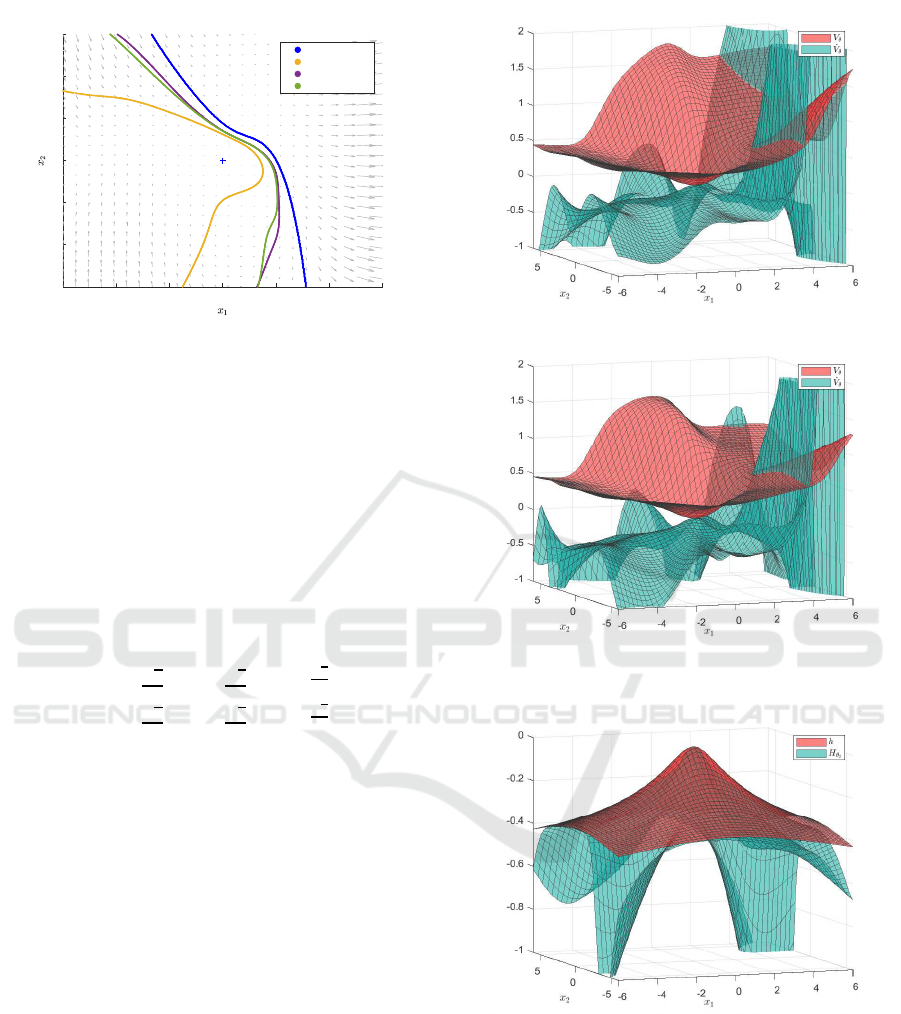
In Figure 1, Regions of Attraction (RoA) of

Lyapunov functions obtained by the single network

method a nd the two-network method, as long as

Hessian-based approach, are compared. The regions

obtained are not included in the display window,

which is limited to the size of X

, as tra je ctories con-

sidered during training may leave the window before

converging to 0. In view of this result, our training

methods can be considered efﬁcient, since they al-

low us to ﬁnd Lyapunov functions with regions of at-

traction close to the true region of attraction. As we

have not precisely optimized the parameter settings,

we can hope that with an hyperparameter optimiza-

tion method we can obtain an even more accura te es-

timate of the tru e Ro A.

Lyapunov functions obtained for th e single-

network method and the two-network meth od, and

their time derivative functions, are respectively d is-

played in Figures 2a and 2b. As can be seen, 0 is a

local minimum for V

, and a local maximum for

on the points grid considered for display.

In order to compare single network and two-

network approachs, Figure 3 shows functions h (10)

and H

(12). As described in section 3, the second

is deﬁned by training, whereas the ﬁr st is not. As we

obtained a similar RoA for the two methods, it is dif-

ﬁcult to conclude he re abou t a possible advantage of

Locally Convex Neural Lyapunov Functions and Region of Attraction Maximization for Stability of Nonlinear Systems

-6 -4 -2 0 2 4 6

-6

-4

-2

Phase plan

True RoA

Hessian

One Network

Two Networks

Figure 1: RoA comparison - Example 1.

using the two-network approach instead of the single

one. However, we can emphasize the supposed ad-

vantage of using it, since H

is visually closer to

in Figure 2b than h to

in Figure 2a. Final values of

cost terms L

(8) and L

′

(13), estimate d for all x ∈ X,

provide a num e rical overview of the difference be -

tween the two approaches. We have L

= 7.7 ×10

−4

and L

′

= 4.4 ×10

−3

, which conﬁrm the visual o bser-

vation. The performance measurement study detailed

in section 4.4 would allow us to conclude.

Example 2.







˙x

= −



−

√





−

√



+ e

−

√

−1

˙x

= −



−

√





−

√



+ e

−

√

−1

(19)

The domain con sidered is X = [−4 ; 4]

and x

[−7.4.10

−3

;−7.4.10

−3

] is a stable equilibrium.

In Figure 4, Regions of Attraction (RoA) of

Lyapunov functions obtained by the single network

method and the two-network method are compared.

The second method seems to be more efﬁcient but we

will see in section 4.4 if it comes from a better random

seed at initialization or a more efﬁcient approach.

Lyapunov functions obtained for th e single-

network method and the two-network method, and

their time derivative functions, are respectively dis-

played in Figures 5a and 5b, and the same co nclusion

as before can be made about their values at the equi-

librium.

Figure 6 shows functions h (10) and H

(12), and

we apply the same argumentation as for example 1.

is visually closer to

in Figure 5b than h to

in Figure 5a. For all x ∈X, we have L

= 0.1531 and

′

= 0.0478, which conﬁrm the visual observation.

We rely on section 4.4 to compare the effectiveness

of the two approache s.

(a) Single Network Approach.

(b) Double Network Approach.

Figure 2: Lyapunov functions comparison - Example 1.

Figure 3: Estimator comparison - Example 1.

4.4 Performance Measurement

Due to the stochastic na ture of our methods, we sub-

ject each system to a series of 50 succ e ssive runs

using the same training data set and different seeds

in o rder to test wheth er their r e sults are parameter-

dependent.

We list the minimum value t

min

, the average value

mean

and the standard d eviation t

std

of the tra ining

ICINCO 2023 - 20th International Conference on Informatics in Control, Automation and Robotics

-4 -3 -2 -1 0 1 2 3 4

-4

-3

-2

-1

Phase plan

True RoA

One Network

Two Networks

Figure 4: RoA comparison - Example 2.

(a) Single Network Approach.

(b) Double Network Approach.

Figure 5: Lyapunov functions comparison - Example 2.

time obtained, the minimum va lue L

min

, the average

value L

mean

and the standard d eviation L

std

of the ﬁ-

nal cost fu nction obtained, as long as the maximum

value D

max

, the average value D

mean

and the standa rd

deviation D

std

of the size of the RoA obtained as a

percentage compared to the size of the initial set X

in Table 3 for the single network method. The same

results are presented in Table 4 for the two-network

Figure 6: Estimator comparison - Example 2.

Table 3: Single Network Approach Performance Measure-

ment.

Benchmarks Example 1 Example 2

min

(s) 21.59 9.49

mean

(s) 22.35 10.77

std

(s) 1.34 2.24

min

6.1 ×10

−3

2.64 ×10

−2

mean

6.6 ×10

−3

3.05 ×10

−2

std

6.8 ×10

−4

1.9 ×10

−3

max

(%) 82.7 71.6

mean

(%) 19.2 32.4

std

(%) 13.35 21.9

method. The results presented in section 4.3 corre-

spond to the D

max

values.

The difference in execution times between the two

examples can be linked to the number of training data

items considered, as shown in Table 2. As the nu mber

of iterations is equally ﬁxed for each run, it is consis-

tent to obtain low standart deviations for L and t.

The evolution of D

mean

between the two ap-

proach e s is signiﬁcant, with an incr ease of 5.5% for

example 1 and 11.9% for example 2, which tends to

validate the advantages of the two-network ap proach.

If the differentiability of the system considered is un-

known or uncertain, the second method is therefore

recommended. Since this approach requires twice the

parameters to be train ed, the average calculation time

is, as expected, the shortcoming.

5 CONCLUSIONS

In conclu sio n, this paper addresses th e challenge

of valid ating Lyapunov proper ties w ithout explicitly

computing the H e ssian eigenvalues and proposes two

approa c hes to so. By app lying them to examples,

the paper demonstrates the effectiveness of the pro-

cess in validating the Lyapunov principle. A c ompar-

Locally Convex Neural Lyapunov Functions and Region of Attraction Maximization for Stability of Nonlinear Systems

Table 4: Two-Network Approach Perf ormance Measure-

ment.

Benchmarks Example 1 Example 2

min

(s) 32.43 16.77

mean

(s) 33.90 18.33

std

(s) 2.33 1.74

min

5.4 ×10

−3

2.53 ×10

−2

mean

5.8 ×10

−3

2.91 ×10

−2

std

3.6 ×10

−4

2.1 ×10

−3

max

(%) 77.1 86.2

mean

(%) 24.7 44.3

std

(%) 15.8 24.5

ison with a Hessian-based approa c h co nﬁrms the efﬁ-

ciency of the proposed training scheme. The ability to

validate Lyapunov functions with out explicitly com-

puting the Hessian pr ovides a valuable alter native, es-

pecially in cases where a differentiable expression of

the system dynamics is not readily available.

This research opens up possibilities for broade r

application of the Lyapun ov princip le , making it more

accessible and applicable in various domains. Further

investigations can explore the extension of those ap-

proach e s to more complex systems and practical sce-

narios, ensuring their robustness and reliability, or can

focus on hyperparameters optimization to increase the

probability to ﬁnd the largest Region of Attra ction for

the system considered.

REFERENCES

Bocquillon, B., Feyel, P., Sandou, G., and Rodriguez-

Ayerbe, P. (2022). A comprehensive framework to

determine lyapunov functions for a set of continuous

time stability problems. In IECON 2022 – 48th An-

nual Conference of the IEEE Industrial Electronics

Society, pages 1–6.

Chang, Y.-C. and Gao, S. (2021). Stabilizing Neural Con-

trol Using Self- Learned Almost Lyapunov Critics. I n

2021 IEEE International Conference on Robotics and

Automation (ICRA), pages 1803–1809.

Chang, Y.-C., Roohi, N. , and Gao, S. (2020). Neural Lya-

punov Control. arXiv:2005.00611 [cs, eess, stat].

Cybenko, G. (1989). Approximation by superpositions of a

sigmoidal function. Mathematics of Control, Signals

and Systems, 2(4):303–314.

Gaby, N., Zhang, F., and Ye, X. (2022). Lyapunov-net: A

deep neural network architecture for lyapunov func-

tion approximation. In 2022 IEEE 61st Conference

on Decision and Control (CDC), pages 2091–2096.

Giesl, P. and Hafstein, S. (2015). R eview on computational

methods for Lyapunov functions. Discrete and Con-

tinuous Dynamical Systems - B, 20(8):2291.

Hornik, K. ( 1991). Approximation capabilities of mul-

tilayer feedforward networks. Neural Networks,

4(2):251 – 257.

Hornik, K., Stinchcombe, M., and White, H. (1989). Multi-

layer feedforward networks are universal approxima-

tors. Neural Networks, 2(5):359 – 366.

Khalil, H. K . (2001). Nonlinear Systems. Pearson, Upper

Saddle River, NJ, 3 edition.

Kingma, D. P. and Ba, J. (2017). Adam: A Method for

Stochastic Optimization. arXiv:1412.6980 [ cs].

Liang, S. and Srikant, R. (2017). Why deep neural net-

works for function approximation? 5th International

Conference on Learning Representations, ICLR 2017

- Conference Track Proceedings.

Matlab (2019). Update parameters using adaptive moment

estimation (Adam) - MATLAB adamupdate.

Mawhin, J. (2005). Alexandr Mikhailovich Liapunov, The

general problem of the stability of motion (1892),

pages 664–676. Elsevier.

Petridis, V. and Petridis, S. (2006). Construction of neu-

ral network based lyapunov functions. IEEE Interna-

tional Conference on Neural Networks - Conference

Proceedings, pages 5059 – 5065.

Prokhorov, D. (1994). A Lyapunov machine for stabilit y

analysis of nonlinear systems. In Proceedings of 1994

IEEE International Conference on Neural Networks

(ICNN’94), volume 2, pages 1028–1031 vol.2.

Richards, S. M., Berkenkamp, F., and Krause, A. (2018).

The Lyapunov Neural Network: Adaptive Stability

Certiﬁcation for Safe Learning of Dynamical Sys-

tems. arXiv:1808.00924 [cs].

ICINCO 2023 - 20th International Conference on Informatics in Control, Automation and Robotics