Enhancing ε-Sampling in the AεSεH

Evolutionary Multi-Objective Optimization Algorithm

Yu Takei

, Hern´an Aguirre

and Kiyoshi Tanaka

Department of Electrical and Computer Engineering, Shinshu University, Wakasato, Nagano, Japan

Keywords:

Many-Objective Optimization, Pareto Dominance Extension, AεSεH, Improving ε-Sampling,

MNK-Landscapes.

Abstract:

AεSεH is one of the evolutionary algorithms used for many-objective optimization. It uses ε-dominance during

survival selection to sample from a large set of non-dominated solutions to reduce it to the required population

size. The sampling mechanism works to suggest a subset of well distributed solutions, which boost the per-

formance of the algorithm in many-objective problems compared to Pareto dominance based multi-objective

algorithms. However, the sampling mechanism does not select exactly the target number of individuals given

by the population size and includes a random selection component when the size of the sample needs to be ad-

justed. In this work, we propose a more elaborated method also based on ε-dominance to reduce randomness

and obtain a better distributed sample in objective-space to further improve the performance of the algorithm.

We use binary MNK-landscapes to study the proposed method and show that it signiﬁcantly increases the

performance of the algorithm on non-linear problems as we increase the dimensionality of the objective space

and decision space.

1 INTRODUCTION

Many real-world problems require that multiple ob-

jective functions be optimized simultaneously. Multi-

objective evolutionary algorithms (Deb, 2001; Coello

et al., 2002) (MOEAs) are a class of algorithms

to solve these problems. MOEAs’ initial suc-

cess brought new challenges as their use became

widespread in numerous application domains.

There are several important areas of ongoing re-

search. Among them, the design of MOEAs to search

effectively and efﬁciently on problems with larger

search spaces, many objective functions, and robust-

ness to distinct shapes of the Pareto front and distinct

geometries of the Pareto set. Performance scalability

of the algorithm when facing increased complexity of

the search space, deﬁned in terms of interacting vari-

ables, is also a challenge to state-of-art MOEAs and

an active research area.

This work deals mainly with manyobjective prob-

lems and increased complexity due to variable inter-

actions. It’s known that the performance of MOEAs

decreases as the objective space dimensionality in-

https://orcid.org/0009-0008-1481-0553

https://orcid.org/0000-0003-4480-1339

creases (von L¨ucken et al., 2019). Several research

efforts based on different approaches aim to improve

evolutionary algorithms for many-objective optimiza-

tion. These include decomposition into several single

objective problems, extensions of Pareto dominance,

and incorporation of performance indicators. It’s also

known that MOEAs’ performance drops when vari-

able interactions increase.

In this work, we focus on an algorithm based on

an extension of Pareto dominance, AεSεH (Aguirre

et al., 2013; Aguirre et al., 2014), and investigate

deeply its survival selection mechanism aiming to im-

prove its performance on many-objective problems

with varying degrees of variable interactions.

AεSεH includes ε-dominance(Laumanns et al.,

2002) for survival selection and parent selection. Dur-

ing survival selection, the algorithm samples from a

large set of non-dominatedsolutions to reduce it to the

required population size. The sampling mechanism

works to suggest a subset of solutions spaced accord-

ing to the ε parameter of ε-dominance, which boost

the performance of the algorithm in many-objective

problems compared to Pareto dominance based multi-

objective algorithms.

However, the sampling mechanism does not select

exactly the target number of individuals given by the

Takei, Y., Aguirre, H. and Tanaka, K.

Enhancing ε-Sampling in the AεSεH Evolutionary Multi-Objective Optimization Algorithm.

DOI: 10.5220/0012181300003595

In Proceedings of the 15th International Joint Conference on Computational Intelligence (IJCCI 2023), pages 86-95

ISBN: 978-989-758-674-3; ISSN: 2184-3236

population size. In most cases there will be a sur-

plus or shortage of non-dominated individuals and an

adjustment to either cut-off or add non-dominated in-

dividuals is requiered. This adjustment process after

sampling is done by random selection in the conven-

tional algorithm. In this work, we improve the ad-

justment process by adding another step based on ε-

dominance to reduce randomness and obtain a better

distributed sample in objective-space to further im-

prove the performance of the algorithm.

We use MNK-landscapes (Aguirre and Tanaka,

2007) as benchmark problems. MNK-landscapes

are binary multi-objective maximization problems,

which can be randomly generated by arbitrarily set-

ting the number of objectives M, the number of de-

sign variables N, and the number of interacting vari-

ables K for each of the variables of the problem.

We conduct experiments on landscapes with M =

{4,5,6, 7} objectives, N = {100,300,500} bits and

K = {5, 6, 10,15,20} epistatic bits. We use vari-

ous metrics to evaluate the non-dominated solutions

found and show that the proposed method signiﬁ-

cantly increases the performance of the AεSεH al-

gorithm on non-linear problems with increased di-

mensionality of the objective space and decision

space. Furthermore, an experimental comparison

with MOEA/D (Zhang and Li, 2007), a well known

MOEA, is included for reference.

2 ADAPTIVE ε-SAMPLING AND

ε-HOOD (AεSεH)

AεSεH is a multi- and many-objective evolution-

ary algorithm that includes mechanisms based on ε-

dominance for survival selection and parent selection.

For survival selection, it uses adaptive ε-Sampling to

expand the dominance region and sample the non-

dominated solution set, which becomes larger as the

number of objectives increases. On the other hand,

Adaptive ε-Hood is used to create neighborhoods in

objective space. When generating offspring, the par-

ents are selected from the same neighborhood.

2.1 ε-Dominance

In AεSεH, the ε-transformation function is applied to

the vector of evaluated values f

f(x

x) of a solution x

x to

transform it into f

′

x). Considering a maximization

problem, we say x

x ε-dominates y

y when the vectors of

transformed values f

′

x) and evaluated values f

f(y

of another solution y

y satisfy the following conditions.

f(x

x) 7→

′

∀i ∈ {1,··· ,M} f

′

x) ≥ f

y) ∧

∃i ∈ {1,··· ,M} f

′

x) > f

y),

(1)

where f

f(x

x) 7→

′

x) is a transformation function

controlled by the parameter ε.

2.2 ε-Sampling

In elitist multi-objective evolutionary algorithms sur-

vival selection is typically performed after joining

the parent and offspring populations. The number of

non-dominated solutions |F

| in this joined population

rapidly surpasses the population size |P|, particularly

when the number of objectives is larger than 3. When

this occurs, the surviving population is a subset of the

non-dominated set of solutions F

. ε-Sampling is a

method designed to obtain a well distributed sample

of non-dominated solutions from F

for the next gen-

eration. In the following we explain the process with

more detail.

1. The individuals in F

with the largest and small-

est evaluation values in each objectiveare selected

for survival, added to the ε-sampled front F

and

deleted from F

2. One individual x

x is randomly selected from F

and f

f(x

x) is transformed to f

′

x) by the ε-

transformation function using the parameter ε

We eliminate from F

the solutions that are ε-

dominated by x

x and add them to a subpopulation

of discarded solutions D. Move x

x to the ﬁrst ε-

front F

3. Step 2 is repeated until F

is exhausted.

4. If |F

| is less than the population size |P| then

|P| − |F

| individuals are randomly selected from

the subpopulation of discarded solutions D and

added to F

. On the other hand, if |F

| is larger

than |P| then |F

| − |P| individuals are randomly

removed from F

The above operations are used to select parent indi-

viduals well distributed in objective space.

2.3 ε-Hood

In AεSεH, ε-Hood is used to divide the parent pop-

ulation P in neighborhoods in the objective space,

and mating partners for recombination are deter-

mined within the neighborhoods(Aguirre et al., 2013;

Aguirre et al., 2014). ε-Hood uses a different parame-

ter ε

than ε-Sampling to generate neighborhood pop-

ulations based on ε-dominance.

Enhancing ε-Sampling in the AεSεH Evolutionary Multi-Objective Optimization Algorithm

2.4 ε-Transformation Function

In this paper, MaxMedian is used as the ε-

transformation for each objective function as shown

below.

′

x) = f

x) + (ε× (max { f

x) : x

x ∈ P}

− median { f

x) : x

x ∈ P}))

(2)

Here, the ε-dominant region is determined by adding

to the ﬁtness value ε multiplied by the difference be-

tween the maximum and median values of the i-th

function.

2.5 Adaptive Changes in ε

The parameters ε

of ε-Sampling is changed adap-

tively at each generation depending on the size of the

set of non-dominated solution sampled by ε-Sampling

NS (before the adjustment) and the population size

|P|.

if NS > |P|

∆ ← min(∆× 2,∆max)

← ε

+ ∆

if NS < |P|

∆ ← max(∆× 0.5, ∆min)

← max(ε

− ∆,0.0) (3)

In this paper, the initial values of ε

and ∆ are set

to ε

= 0.0, ∆

= 0.005, ∆ to ∆

max

= 0.1, ∆

min

0.0000001.

To adapt ε

for ε-Hood we follow a similar pro-

cedure, comparing the created number of neighbor-

hoods with a desired number speciﬁed by the user

(Aguirre et al., 2013).

3 AεSεH SHORTCOMING

ε-Sampling does not select exactly the target number

of individuals from the set of non-dominated solu-

tions. In most cases there will be a surplus or shortage

of individuals and an adjustment to either cut-off or

add individuals will be done by random selection to

achieve the target number of individuals (section 2.2,

Step 4). To illustrate this, after ε-Sampling is per-

formed, the degree of random selection is checked by

actually solving MNK-landscapes test problem. The

parameters given to the MNK-landscapes and evolu-

tionary algorithm are shown in Table 1 and Table 2.

For each value of M, the same MNK-landscape is

solved 30 times from different random initial popu-

lations. Two-point crossover and bit-ﬂip mutation are

used as operators.

Table 1: Parameters of MNK-landscapes.

Parameters Value

Number of Objectives M 4, 5, 6, 7

Number of Variables N 100

Number of Interacting Variables K

Variables Interaction Random

Table 2: Parameters of EA.

Parameters Value

Generations G 10,000

Population Size |P|

200

Mutation Ratio P

1/N

Figure 1 shows the number of non-dominated in-

dividuals before and after ε-Sampling, averaged over

30 trials for each generation. As expected, note that

the number of pre-sampled non-dominated solutions

increased with the dimensionality of the objective

space. Looking at the difference between popula-

tion size and the number of solutions after sampling,

note that the application of ε-Sampling resulted in the

random selection of less than 25 individuals for four

objectives and approximately 50 individuals for ﬁve

and more objectives. From the above, it can be seen

that there is always a random part in the selection of

surviving individuals by ε-Sampling, which increases

with the number of objectives. In the problem set up

for this experiment, this increase in random selection

is particularly noticeable when the number of objec-

tives increased from four to ﬁve.

Figure 1: Average number of individuals before and after

ε-Sampling. Top 4 objectives, bottom 5 objectives.

ECTA 2023 - 15th International Conference on Evolutionary Computation Theory and Applications

It is likely that the individuals randomly selected

may disrupt the adequately spaced populations ob-

tained by ε-Sampling. In the next section, we propose

a method that aims to enhance ε-Sampling by select-

ing all individuals appropriately spaced.

4 PROPOSED METHOD

4.1 Reducing Randomness in Survival

Selection

As a method to reduce the random selection in ε-

Sampling, we consider applying ε-dominance again

after ε-Sampling to a reference subpopulation of non-

dominated solutions (explained with detail in section

4.2). In this case, a different ε-transformation func-

tion is used with a new ε, in addition to the expan-

sion ratio ε

adapted throughout all the generations in

ε-Sampling. The new ε is computed by estimating

the mean distance in objective space of the top-rating

individuals. Several iterations of sampling over in-

creasingly smaller reference subpopulations, resetting

ε appropriately, are repeated until the target number

of individuals is reached. This method is expected to

achieve better uniformity in the selected sample than

the conventional method.

In the following we deatil the main steps of the

proposed method. The procedure receives a reference

set of solutions R from which a target number N

must

be sampled, i.e. |R| − N

solutions must be deleted

from R. It returns a sample S ∈ R of size |S| = N

1. Set the iteration counter k ← 1 and the maximum

number of iterations T. Also, set the initial sam-

pling population R

← R and save its size for ref-

erence N

← |R|.

2. Set a base expansion value u

for each

one of the M objective functions, u

←

,··· ,u

) according to the distribu-

tion of R

. Set the sample to empty, S

← ∅. Set

the set of discarded solutions to empty, D

← ∅.

3. Select one solutiom x

x randomly from R

and

transform its vector of ﬁtness values f

f(x

x) to f

′

using u

and ε

. Use the f

′

x) vector to compute

ε-dominance between x

x and the other solutions in

. Remove solutions in R

that are ε-dominated

by x

x and add them to the set D

of discarded solu-

tions. Remove x

x from R

and add it to the set S

of sampled solutions.

4. Repeat Step 3 if R

6= ∅ (not empty). Otherwise,

continue with Step 5.

5. If |S

| > N

and k < T then resample from S

; that

is, increase the iteration counter k ← k+ 1, set the

new current sampling population R

← S

k−1

. Up-

date the expansion rate ε

← ε

k−1

× ∆ and repeat

from Step 2. Otherwise, continue to Step 6.

6. If the sample size is not exactly equal to the num-

ber required then adjust the sample size randomly.

That is, if |S

| > N

eliminate randomly |S

| − N

solutions from S

. Otherwise, if |S

| < N

, select

randomly N

− |S

| solutions from the current set

of discarded solutions D

and add them to S

7. Return S

The base expansion value u

at the k-th iteration of

the procedure for the i-th ﬁtness function is computed

as shown in (4) below.

=(max { f

x) : x

x ∈ R

}

− median { f

x) : x

x ∈ R

})/(

+ 1)

(4)

where n

is the number of individuals in the sampling

population R

, max

and median

are the maximum

and median values in the i-th objective function com-

puted from R

. The ε-transformation function at the

k-th iteration to expand the i-th ﬁtness value of the

solution is as shown in (5) below.

′

x) = f

x) + u

× ε

(5)

where u

is the base expansion value and ε

is the

expansion rate.

As mentioned above, the expansion rate ε

is up-

dated at each iteration k of the procedure as shown in

(6) below.

= ε

k−1

× ∆

= 1

∆ = 1.05,

(6)

where the constat ∆ > 0 works to increase ε

at each

iteration to prevent the number of iterations from be-

coming too large.

Note that for the base expansion u

in (4) we

use a value slightly smaller than the average dis-

tance between the top-rating individuals in the i-th

objective. This means that the individuals eliminated

by ε-dominance when ε

= 1 are those whose inter-

individual distance in objective space is closer than

the mean of the top-rating individuals.

In this paper, experiments are conducted with the

maximum number of iterations T = 100. Regard-

ing the time complexity of the proposed method, the

lower bound is 0 (when the sample size given by

ε-Sampling equals the population size) and the up-

per bound is given by |R|

× T. Box plots of the

actual number of iterations k < T required by the

Enhancing ε-Sampling in the AεSεH Evolutionary Multi-Objective Optimization Algorithm

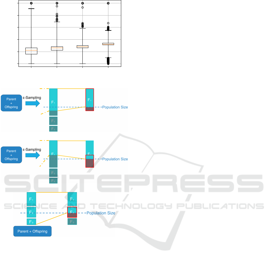
4 5 6 7

The Number of Objectives M

100

The Iteration Counter k

Figure 2: The iteration counter k for each objectives.

(a) Surplus of individuals by ε-Sampling.

(b) Shortage of individuals by ε-Sampling.

Figure 3: Cases where the proposed method will be used.

proposed method are shown in Figure 2 for M =

{4,5,6, 7},N = 100 and K = 5 computed over 10,000

generations and 30 runs of the algorithm. Note that

the median k falls between 20 and 30 iterations.

4.2 Cases in Which the Proposed

Method Will be Used

Depending on the number of individuals after ε-

Sampling is performed, the proposed method can be

applied to the three different cases illustrated in Fig-

ure 3 and listed below.

4.2.1 Selection in Case of Surplus

If the number of individuals sampled by ε-Sampling

exceeds the target population size, the proposed

method is performed on the sample provided by ε-

Sampling as shown in Figure 3a. Then, the sample

returned by the proposed method becomes the popu-

lation for the next generation.

4.2.2 Selection in Case of Shortage

If the number of individuals sampled by ε-Sampling

is less than the target number, the proposed method

is performed on the sub-population of non-dominated

individuals initially discarded by ε-Sampling as

shown in Figure 3b. Then the sample provided by

ε-Sampling and the one returned by the proposed

method are joined to form the population for the next

generation.

4.2.3 Selection in Lower Front

If the number of individuals in the top front is less

than the target number, ε-Sampling is not performed.

In this case, the top fronts are allowed to survive, and

the proposed method is performed on the last front

that overﬂowed the size of the surviving population

as shown in Figure 3c. The sample returned by the

proposed method is joined to the top fronts to form

the population for the next generation.

5 EXPERIMENTAL METHOD

AND EVALUATION

INDICATORS

5.1 Experimental Method

To examine in detail the effects on solution search by

the proposed method, we ﬁrst solve MNK-landscapes

(Aguirre and Tanaka, 2007) varying M from 4 to 7

ﬁxing N = 100 and K = 5 and starting from 30 ini-

tial populations generated with different seeds. The

parameters and other conditions used in the experi-

ments are the same as those used in Table 1 and Ta-

ble 2. Next, we perform experiments varying N =

{100, 300,500} and K = {5, 6, 10,15,20}.

In order to objectively evaluate the proposed

method, we also compare the results with those ob-

tained by MOEA/D (Zhang and Li, 2007), a represen-

tative decomposition based multi-objectiveevolution-

ary algorithm often applied for many-objective opti-

mization. In this experiment, the scalarization func-

tion of MOEA/D is Tchebycheff,which is suitable for

ECTA 2023 - 15th International Conference on Evolutionary Computation Theory and Applications

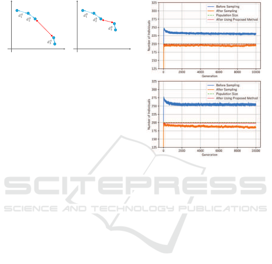
(a) Population A (b) Population B

Figure 4: Example of populations with equal SP.

nonlinear discrete problems, and the neighborhood

size is set to the commonly used value of 20.

The evaluation indexes shown in the next section

are used to evaluate the sets of solutions found by the

algorithms.

5.2 POS Evaluation Indicators

In this study, to evaluate the Pareto optimal solutions

set (POS) obtained by the optimization algorithm, we

use the Hypervolume (HV) (Zitzler, 1999; Fonseca

et al., 2006). To validate the features of the obtained

POS, we also use the Coverage-metric (C-metric),

Overall Pareto Spread (OS), Spacing (SP), and Distri-

bution Metric (DM) (Audet et al., 2021; Zheng et al.,

2017).

Note that the distribution of solutions may cause

problems in the calculation of SP. Consider two

populations that satisfy (d

) = (d

) as

shown in Figure 4. Note that these two populations

clearly have different homogeneity, but when looking

at the distance d

to the nearest solution used to calcu-

late SP, they have exactly the same value. That is, SP

calculated from these values will be exactly the same.

Thus, large distances between multiple neighborhood

groups, such as in Figure 4a, cannot affect the value

of SP and therefore it becomes an unreliable metric in

these situations. DM is an indicator to measure diver-

sity that does not suffer the problem observed in SP

calculation.

6 RESULTS AND DISCUSSION

6.1 Changes in the Actual Number of

Selected Individuals

First, we verify the number of individuals before sam-

pling, after selection by ε-Sampling, and after apply-

ing the proposed method, averaged over 30 trials for

each generation. Results are shown in Figure 5. It

can be seen that the proposed method is able to se-

Figure 5: Population averages before and after ε-Sampling

and after applying the proposed method. N = 100,K = 5,

top 4 objectives, bottom 5 objectives.

lect most of the individuals that were randomly se-

lected by the conventional method i.e. pink line is

similar to the population size shown in green. Com-

paring the number of individuals after sampling with

that of the conventional method shown in Figure 1, it

can be seen that when the proposed method is used ε-

Sampling selects samples which size are closer to the

target number for all numbers of objectives (orange

line). In other words, ε-dominance performed after ε-

Sampling, in addition to reducing randomness, helps

improve ε-Sampling itself.

6.2 POS Evaluation

Next, we evaluate the POS using the indicators listed

above and compare results by the conventional and

proposed method every 1,000 generations using box-

and-whisker diagrams. Welch’s t-test is performed for

the evaluation values of the last generation to deter-

mine if there is a signiﬁcant difference between the re-

sults of the conventional and proposed methods based

on the obtained p-values included in Table 3.

Figure 6 shows the HV over the generations by

AεSεH and its improved version with the proposed

method. These plots and the p-values of the HV row

in Table 3 show that in terms of HV there is a sig-

niﬁcant difference in performance by both algorithms

for ﬁve or more objectives, and that performance im-

Enhancing ε-Sampling in the AεSεH Evolutionary Multi-Objective Optimization Algorithm

Figure 6: HV obtained in 30 runs. N = 100,K = 5, left to right, top 4, 5 objectives and bottom 6, 7 objectives.

Figure 7: C-metric meassured in 30 runs. N = 100,K = 5, left to right, top 4, 5 objectives and bottom 6, 7 objectives.

Table 3: p-value in the last generation.

Ind.

Number of Objectives M

4 5 6 7

HV 8.62e-01 2.18e-04 1.41e-11 1.81e-14

C 6.80e-03 4.53e-07 1.05e-06 4.07e-11

OS 6.53e-01 6.44e-01 4.40e-01 1.94e-01

SP 1.56e-04 2.64e-06 2.94e-06 9.91e-02

DM 3.85e-01 1.19e-02 2.42e-01 2.25e-01

proves as the number of objectives increases.

Figure 7 shows results by the C-metric.

C(AεSεH,Improved) represents the proportion

of the POS found by the proposed method that is

dominated by the POS found by the conventional

method, and C(Improved,AεSεH) represents the

opposite. The results show that convergence im-

proved for all objectives tested, and this difference

becomes more signiﬁcant as the number of objectives

ECTA 2023 - 15th International Conference on Evolutionary Computation Theory and Applications

Figure 8: SP meassured in 30 runs. N = 100,K = 5, left to right, top 4, 5 objectives and bottom 6, 7 objectives.

increases. The p-values for the C-metric in Table 3

support this.

The p-values for the OS in Table 3 show that there

is no statistical difference on spread by both methods.

This is because the solutions with maximum and min-

imum evaluation values for each objective are kept,

which is performed before applying ε-Sampling.

Figure 8 shows results on spacing computing SP.

From Table 3, we can see that there is a signiﬁcant

difference in SP except for 7 objectives. In addition,

the mean and variance are considerably smaller by the

proposed method for all numbers of objectives as can

be observed in Figure 8, which indicates that the uni-

formity is better in the proposed method.

The p-values for the DM in Table 3 show that no

clear statistical differences between the two methods

for DM.

6.3 Discussion

There is a statistically signiﬁcant improvement in HV

by the proposed method for many objectiveproblems.

To have a better understanding on the effects of the

proposedmethod and determine whether the improve-

ment is due to convergence or diversity we looked to

other metrics.

First, C-metric shows that the convergence of

POS improves regardless of the number of objectives.

Also, the convergencedifference between the conven-

tional and proposed methods becomes larger as the

number of objectives increases. Next, in terms of di-

versity, there was no difference in spread (OS), and

while there was an improvement and stabilization in

terms of uniformity (SP), there was no improvement

in overall diversity (DM). This may be due to the

aforementioned shortcomings of SP. While SP can

only evaluate local uniformity, DM evaluates the di-

versity of the entire distribution of solutions. This in-

dicates that the diversity has not improved when look-

ing at the set of non-dominated solution as a whole,

but it has improved locally. In other words, although

uniformity is improved within groups of neighbor so-

lutions, there is distance between the groups, and the

distribution cannot be said to be uniform when viewed

across the entire objective space.

From the above, it can be inferred that the solution

search performance for each neighborhood improves

as a result of better local uniformity, which improves

the convergence of the solution group as a whole.

Given that there is a correlation between the increase

in the number of objectives and the improvement in

convergence, uniform solution search becomes more

important as the dimension of the objective space ex-

pands.

The fact that the proposed method also improves

the accuracy of ε-Sampling as a side effect was re-

vealed from the visualization of the actual selection

of the proposed method. This is due to the improved

uniformity of the solution distribution, which allows

a more precise estimation of ε

between generations.

Enhancing ε-Sampling in the AεSεH Evolutionary Multi-Objective Optimization Algorithm

Table 4: p-value in the last generation for each N.

4 5 6 7

100 8.62e-01 2.18e-04 1.41e-11 1.81e-14

300 6.10e-06 8.16e-09 8.70e-12 9.63e-15

500 1.34e-06 7.67e-08 8.71e-12 1.88e-13

Figure 9: HV obtained at the last generation in 30 runs vary-

ing the number of variables N. M = 6,N = {100,300,500}

and K = 5.

6.4 Comparison Varying N and K

In this section we verify the performance of the pro-

posed method increasing the complexity of the prob-

lem and the dimension of the search space.

Figure 9 shows results for M = 6 objectives and

K = 5 bits, N from 100 to 500. Note that the pro-

posed method performs signiﬁcantly better than the

conventional approach when we increase the size of

the search space. In addition, note that the variance is

smaller by the proposed method. This is corroborated

by the p-values in Table 4, which also includes results

for other values of M.

Table 5: p-value in the last generation for each K.

4 5 6 7

5 8.62e-01 2.18e-04 1.41e-11 1.81e-14

6 9.77e-01 1.35e-05 4.56e-14 8.58e-16

10 1.57e-01 6.78e-03 1.55e-10 1.28e-14

15 3.57e-01 3.41e-02 1.60e-05 4.05e-10

20 4.23e-01 1.80e-01 4.08e-03 3.88e-04

Figure 10 shows results for M = 6 objectives and

N = 100 bits, varying K from 6 to 20. Note that

the proposed method performs signiﬁcantly better in

a broad range of K and that the advantage gradually

decreases as K increases. The reason why the perfor-

mance for K = 20 by both methods become similar is

that the number of sampled solutions by ε-Sampling

approaches the desired population size, as shown in

Figure 11, leaving little room for the proposed method

Figure 10: HV obtained at the last generation in 30 runs

varying the number of interacting variables K. M = 6,N =

100 and K = {5,6, 10,20}.

Figure 11: Average number of individuals before and after

ε-Sampling. M = 6,N = 100, top K = 10, bottom K = 20.

to improve the sample. Similar results in favor of the

proposed method are observed with other values of M

when we vary K, as corroborated by the p-values in

Table 5.

6.5 Comparisson with Other MOEA

Decomposition based algorithms are being broadly

used for many-objective optimization. To illustrate

the relative performance of the improvedAεSεH with

respect to these kind of algorithms, we also conduct

experiments with MOEA/D, a well known decompo-

sition based algorithm. Figure 12 shows the transi-

tion of the HV over the generations by the improved

AεSεH and MOEA/D on M = 5,6 objectives, N =

100 bits and K = 5 epistatic interactions. From the

ﬁgure we can see that the improved AεSεH achieves

a signiﬁcantly better HV than MOEA/D. Note that

ECTA 2023 - 15th International Conference on Evolutionary Computation Theory and Applications

Figure 12: Comparisson with MOEA/D. K = 5,N = 100,

top 5 objectives, bottom 6 objectives.

the performance of the proposed algorithm at the

2,000th generation is already better than MOEA/D at

the 10,000th generation.

7 CONCLUSIONS

In this study, we focused on the ε-Sampling part of

Adaptiveε-Sampling and ε-Hood (AεSεH) algorithm,

and conﬁrmed through experiments that AεSεH per-

forms better solution search with the improved pro-

posed method. This performance improvement was

more pronounced as the number of objectives in-

creased. This is attributed to the increased impor-

tance of a search process that emphasizes solution

uniformity in response to the expansion of the objec-

tive space as the number of ﬁtness functions increase.

Since AεSεH is an algorithm developed for multi-

and many-objective optimization, this improvement

reinforces its many-objective characteristics. We also

found that improving solution uniformity leads to

the generation of solution distributions that are more

prone to ε-Sampling with high accuracy. In addition,

we showed that AεSεH scales up well with the di-

mension of the search space and complexity of the

problem.

In the future, we would like to explore dynamic

schedules for the ampliﬁcation factor in the proposed

scheme, reﬂecting, for example, the size of the tar-

get population and the number of target individuals,

which would not only further reduce randomness but

also reduce the number of calculations.

REFERENCES

Aguirre, H., Oyama, A., and Tanaka, K. (2013). Adap-

tive ε-Sampling and ε-Hood for Evolutionary Many-

Objective Optimization. In Evolutionary Multi-

Criterion Optimization (EMO 2013). Lecture Notes

in Computer Science, volume 7811, pages 322–336.

Springer Berlin Heidelberg.

Aguirre, H., Yazawa, Y., Oyama, A., and Tanaka, K.

(2014). Extending AεSεH from Many-objective to

Multi-objective Optimization. In Simulated Evolution

and Learning (SEAL 2014). Lecture Notes in Com-

puter Science, volume 8886, pages 239–250. Springer,

Cham.

Aguirre, H. E. and Tanaka, K. (2007). Working Princi-

ples, Behavior, and Performance of MOEAs on MNK-

landscapes. European Journal of Operational Re-

search, 181(3):1670–1690.

Audet, C., Bigeon, J., Cartier, D., Le Digabel, S., and Sa-

lomon, L. (2021). Performance Indicators in Multi-

objective Optimization. European Journal of Opera-

tional Research, 292(2):397–422.

Coello, C., Van Veldhuizen, D., and Lamont, G. (2002).

Evolutionary Algorithms for Solving Multi-Objective

Problems. New York, Kluwer Academic Publishers.

Deb, K. (2001). Multi-Objective Optimization using Evolu-

tionary Algorithms. John Wiley & Sons.

Fonseca, C. M., Paquete, L., and L´opez-Ib´anez, M.

(2006). An Improved Dimension-Sweep Algorithm

for the Hypervolume Indicator. In 2006 IEEE In-

ternational Conference on Evolutionary Computation,

pages 1157–1163. IEEE.

Laumanns, M., Thiele, L., Deb, K., and Zitzler, E. (2002).

Combining Convergence and Diversity in Evolution-

ary Multiobjective Optimization. Evolutionary Com-

putation, 10(3):263–282.

von L¨ucken, C., Brizuela, C., and Bar´an, B. (2019).

An Overview on Evolutionary Algorithms for Many-

Objective Optimization Problems. Wiley Interdisci-

plinary Reviews: Data Mining and Knowledge Dis-

covery, 9(1):e1267.

Zhang, Q. and Li, H. (2007). MOEA/D: A Multiobjec-

tive Evolutionary Algorithm based on Decomposi-

tion. IEEE Transactions on Evolutionary Computa-

tion, 11(6):712–731.

Zheng, K., Yang, R.-J., Xu, H., and Hu, J. (2017). A

New Distribution Metric for Comparing Pareto Opti-

mal Solutions. Structural and Multidisciplinary Opti-

mization, 55:53–62.

Zitzler, E. (1999). Evolutionary Algorithms for Multiobjec-

tive Optimization: Methods and Applications. PhD

thesis, Diss. ETH No 13398, Swiss Federal Institute

of Technology Zurich.

Enhancing ε-Sampling in the AεSεH Evolutionary Multi-Objective Optimization Algorithm