Using Abstraction Graphs to Promote Exploration in Curiosity-Inspired

Intrinsic Motivation

Mahtab Mohtasham Khani

, Kathryn Kasmarik

, Shadi Abpeikar

and Michael Barlow

UNSW Canberra, University of New South Wales, Canberra, Australia

Keywords:

Intrinsically Motivated Reinforcement Learning, Graph Representation, Computer Game, Curiosity Models.

Abstract:

This paper proposes a new approach to modelling IM using abstraction graphs to create a novel curiosity

model. An abstraction graph can model the topology of a physical environment in a manner that is not captured

by typical curiosity models that use self-organising or adaptive resonance theory networks. We hypothesise

that this can permit more systematic exploration and skill development in a motivated reinforcement learning

setting. To evaluate the proposed model, we have compared our agent’s behaviour with an existing curiosity

model in the same environment and the same conﬁguration. For this evaluation, we examined each agent’s

behaviour at different life stages and characterised the exploration and attention focus of each agent in each

life stage. We concluded the best uses of each approach.

1 INTRODUCTION

Reinforcement learning (RL), permits an agent to

learn skills through a trial-and-error procedure (Sut-

ton and Barto, 1998). Intrinsically Motivated RL

(IMRL) is an approach to the progressive acquisition

of behavioural competence for RL agents (Peng et al.,

2019). In recent years, there has been a growing ac-

knowledgment that RL agents operating in complex

environments should possess the capability to drive

their own learning. This is due to the recognition

that it is often impractical for system designers to pre-

deﬁne a generic reward signal in advance (Clements

et al., 2019). In various applications, agents en-

counter problems within their environment that may

not be fully known or easily solvable during the ini-

tial training phase. On the other hand, if the agent

acquires knowledge about the environment or its own

capabilities, it can become capable of facing these

new problems in the future without the need for pre-

programming (Din and Caleo, 2000).

Curiosity models have provided an approach to

dynamic reward signals suitable for adapting the at-

tention focus of IMRL agents over the course of their

life. However such models can result in repetitive be-

https://orcid.org/0000-0003-4811-072X

https://orcid.org/0000-0001-7187-0474

https://orcid.org/0000-0002-8404-0290

https://orcid.org/0000-0002-7344-4302

haviour when curiosity is not offset by adequate struc-

tural memory of the agent’s environment. The uti-

lization of graph theory, on the other hand, provides

a powerful tool for abstracting complex learning en-

vironments. Notably, RL with extrinsic and intrin-

sic goals are some instances of these complex learn-

ing environments, that have beneﬁted from the advan-

tages of graph representation theory in recent years

(Huang et al., 2019).

Early work used a range of reward functions simu-

lating concepts such as curiosity and novelty-seeking

behaviour in IMRL (Merrick and Maher, 2009). The

three contributions of this paper are: First, a method

for constructing a graph-based representation of agent

experiences online during lifelong learning. Second,

two IM models make use of this graph representation

to calculate rewards online. And third, metrics for

analysing lifelong learning in terms of the life stages

of an agent.

2 LITERATURE REVIEW

This section brings together literature from four

ﬁelds. Curiosity models, intrinsically motivated RL,

data structure motivation methods, and graph-theory

in RL, to clarify the research niche for this paper.

Mohtasham Khani, M., Kasmarik, K., Abpeikar, S. and Barlow, M.

Using Abstraction Graphs to Promote Exploration in Curiosity-Inspired Intrinsic Motivation.

DOI: 10.5220/0012181400003595

In Proceedings of the 15th International Joint Conference on Computational Intelligence (IJCCI 2023), pages 505-513

ISBN: 978-989-758-674-3; ISSN: 2184-3236

505

Curiosity Inspired Models. Curiosity-inspired

motivation models, with the deﬁnition of IM and

curiosity-driven exploration (Marsland et al., 2005),

play a crucial role in driving agents to explore their

environment. These models focus on modelling the

agent’s drive to explore its environment and seek

out new information (Pathak et al., 2017). They are

based on the idea that the agent is driven by a desire

to reduce its uncertainty about its environment and

use metrics such as prediction error or surprise to

quantify this uncertainty (Pathak et al., 2017).

Intrinsically Motivated RL. In recent years, there

has been increasing recognition that RL agents in

complex environments must be able to drive their own

learning since it is not possible for the system de-

signer to specify a reward signal in advance that is ad-

equate for ongoing lifelong learning (Clements et al.,

2019). In much of the research with IM, there is an ex-

ternal main goal available in the environment and an

architecture that helps to deﬁne different efﬁcient sub-

goals for learning skills and reaching the main goal

(Aubret et al., 2021). This provides advantages in ap-

plications such as computer games where deﬁning in-

trinsic and extrinsic goals can permit faster solutions

to difﬁcult problems (Bellemare et al., 2016).

Also, if the agent learns about the environment,

the properties inside the environment, how impor-

tant these properties are, how its actions can change

the environment, and its own abilities it may be able

to solve new problems in future without being pre-

programmed for them (Din and Caleo, 2000).

Data Structures Motivation Models. Clustering-

based curiosity models are a class of models that use

clustering algorithms to generate curiosity-driven be-

haviours in agents. By clustering their input data,

curiosity models are able to help an agent identify

new goals (and eventually skills) associated with each

identiﬁed cluster(Pathak et al., 2017).

Researchers have developed different unsuper-

vised clustering algorithms, such as k-means clus-

tering (Marsland et al., 2005), self-organizing maps

(SOMs) (Kohonen, 2012), growing neural gas (GNG)

(Fritzke, 1995), grow-when-required (GWR) net-

works (Marsland et al., 2005), adaptive resonance

theory (ART) networks (Grossberg, 1976), and Sim-

pliﬁed ART (SART) networks (Baraldi et al., 1998).

Several of these have been used in curiosity models.

The choice of clustering algorithm for a particular ap-

plication depends on the speciﬁc requirements of the

task.

Self-organising maps (SOMs) are a popular ap-

proach to building clustering-based curiosity models

as they provide dimensionality reduction (Marsland

et al., 2005) while preserving the topological struc-

ture of the input data. It is a type of unsupervised

neural network that can cluster similar input data into

discrete categories (Skupin et al., 2013). The quanti-

zation error (quant

) is a measure to calculate the dis-

tance between each data input and its corresponding

best matching unit (BMU). It measures the degree of

mismatch between the SOM and the input data (Tu,

2019). If the quant

is small, the SOM feature map

will be assessed with good quality.

In this work, we have employed SOM-based cu-

riosity in two ways. We utilized it as a baseline for

understanding the performance of frontier-based IM.

Table 1 shows the details of each clustering al-

gorithm discussed above. In this table, we compare

abstraction graphs to show the differences and sim-

ilarities between existing clustering approaches and

motivate the work in this paper.

Graph Theory in RL. Graph theory has been ap-

plied to a range of problems such as search algo-

rithms (Jin et al., 2021). Some approaches try to ﬁnd

efﬁcient sub-goals for an agent(Jin et al., 2021) by

ﬁnding a high-level plan and using low-level policies

to reach the goal or the sub-goal..Graph theory has

also been applied for action space reduction (Eysen-

bach et al., 2019), and understanding the RL theory

(Buabin, 2013). Some works apply graph abstraction

to both intrinsically and extrinsically motivated RL

methods (Jin et al., 2021).However, none of these ap-

proaches uses graph representation with the purpose

of complementing curiosity which is our focus in this

paper.

3 METHODOLOGY

In this paper, we propose three motivation meth-

ods using abstraction graphs and examine their im-

pact on the behaviour of an agent. In Subsection

3.1, we explain how we create our abstraction graph

while the agent interacts with its environment. Next,

we describe our proposed Frontier-based IM method

in Section 3.2. In this Section, we talk about the

other motivation method which is SOM-based curios-

ity in IMRL. Finally, we propose a Hybrid Frontier-

curiosity algorithm in IMRL.

3.1 Abstraction Graphs

In this section, we will describe the proposed state-

transition graph for representing IM behaviours. In

graph theory, we deﬁne each graph by G = (V,E)

NCTA 2023 - 15th International Conference on Neural Computation Theory and Applications

506

Table 1: Clustering-based Curiosity Models.

Algorithm Prototypes Topology Cluster Initialization Grow Limitations Distance

Metric

SOMs(Kohonen,

2012)

Fixed Topology-preserving (in-

cludes neighbourhood rela-

tions but edges don’t have

meaning)

Randomized, then re-

ﬁned over time

No Not designed for

online learning, can

become saturated

over time

Euclidean

K-Means Clustering

(Marsland et al.,

2005)

Fixed No topology Randomized, then re-

ﬁned over time

No Not topology-

preserving

Euclidean

ART Net-

works(Grossberg,

1976)

Variable No topology Empty at start, popu-

lated over time

Yes Limited to binary

and analog inputs

Hamming

SART Net-

works(Baraldi

et al., 1998)

Variable No topology Empty at start, popu-

lated over time

Yes No neighborhood

relations

Hamming

GNG(Fritzke, 1995) Variable Topology-preserving (in-

cludes neighborhood rela-

tions)

Empty at start, popu-

lated over time

Yes Delay in creating

new cluster proto-

types

Euclidean

GWR Net-

works(Marsland

et al., 2005)

Variable Topology-preserving(includes

dynamically created connec-

tions between nodes)

Empty at start, popu-

lated over time

Yes Can struggle with

high-dimensional

data

Euclidean

Abstraction Graph Variable Topology-preserving (with

edges representing transition)

Populated over time Yes May become large

where G denotes the graph, V represents the vertex

set, and E represents the edge set. In this work, our

graph is represented by G = (S,T), where S repre-

sents different states as different vertexes and T rep-

resents the transition between vertexes. We deﬁne

each transition as the movement of the agent from

state S to state S

′

driven by action A. Initially, we

start with an empty graph represented as G = (

0).

As we progress step by step, we construct our graph

by adding individual states and their corresponding

transitions to it. Equation 1 illustrates the process of

combining states and transitions to form the graph.

Here, S

t−1

represents previous state, S

represents new

states, T

t−1

denotes the transitions from the previous

state, and T

denotes the new transitions.

G = (S

t−1

∪ S

t−1

∪ T

) (1)

In this equation, the union symbol (∪) is used to com-

bine sets, representing the addition of new elements

to the existing sets.

Our Graph abstraction employs multigraphs to

capture parallel or overlapping transitions between

states. The ﬂexibility of multigraphs enables us to ex-

tract the exact degrees of connectivity for each node

which plays a crucial role in the IM algorithms for our

agents.

3.2 IMRL Methods

Algorithm 1 shows the core structure shared by all the

methods presented in this paper. Each method stands

out based on how it calculates the reward, depending

on how it is motivated. This difference makes each

method unique.

Data: environment, n episodes, n runs

Result: G, Q-table

for each run do

Instantiate environment and agent;

Instantiate an empty state transition graph

G = (

0);

for each episode do

while Agent not terminated AND the

step limits are not reached do

Observe the environment in the

step;

Choose the next action based on

an ε − greedy policy;

Update SOM;

Calculate R based on

Equations 3, 5, or 4 accordingly;

Update Q-table using Equation2;

Update G using Equation1;

Take the chosen action;

end

Algorithm 1: Core structure algorithm for all the proposed

methods.

We will describe each method using Algorithm 1

and the different IM methods leading in different re-

Using Abstraction Graphs to Promote Exploration in Curiosity-Inspired Intrinsic Motivation

507

ward functions, in the following.

q[S,A] = q[S,A]+α ∗(R)+λ∗max(q[S

′

])−q[S,A])

(2)

Frontier-Based IMRL. Here we propose our

Frontier-based IMRL method using Algorithm 1 and

calculating the reward function through Equation 3.

Ds in this equation represents the degree for the cur-

rent state.

In the Frontier method, the agent can observe the

current state of the environment as a feature vector.

The record of state transitions of the agent will be

saved in another variable called

′

State − Transition

′

The degree of each state is determined by counting the

number of edges that pass through any speciﬁc node.

In each step of each episode, the agent will ob-

serve the environment and choose the action accord-

ing to the ε − greedy policy. The agent will calculate

the degree of each state if it is more than 0 the intrin-

sic reward of M =

Degree

will be sent to the bellman

equation 2 (Sutton and Barto, 1998) for calculating

the updated Q-value. If the agent visits a new node

with no connections, we can’t calculate the reward as

it leads to M =

which is an error. So, we simply

give it a reward of 1.

R =



1/Ds Ds > 0

1 Ds ≤ 0

(3)

SOM-Based Curiosity in IMRL. As mentioned

previously, we use a SOM-based technique as a base-

line for evaluating our proposed abstraction graph ap-

proach in this paper.

Algorithm 1 will be updated by the SOM IM.

The reward in this method will be calculated through

equation 4. quant

s here means the amount of quanti-

sation error in the current state of S. It replaces the re-

ward component with a −quant

, calculated based on

the current state obtained from the SOM. The quant

is used as an intrinsic reward for the agent which

yields a traversing graph of an agent, dependent on

the SOM. The idea is to analyse and compare the be-

haviour of an RL agent with clustering motivation (by

a negative amount of quant

as the reward) with our

other agents like the Frontier, and the Hybrid Frontier

methods.

At each step of this method, the agent chooses the

next action based on an ε-greedy policy, updates the

SOM, and calculates the quant

for the current state

representation. As we are looking to minimize the

amount of error, we will send the negative form of

quant

as the intrinsic reward to the agent(R). The

Q-table is then updated using the Bellman equation 2

with R as the reward component. Using the quant

as the intrinsic reward, the agent is encouraged to ex-

plore areas closer to the centroid of SOM clusters or

far from the clusters’ boundaries.

R = −quant

s (4)

Hybrid Frontier-Curiosity in IMRL. In this sec-

tion, we propose a hybrid approach that combines

both frontier and curiosity-based IM. We reduce the

value of the quant

of SOM from the Frontier method

and return this value as the reward of our RL agent.

The agent navigates in our proposed grid environment

and in each step, the agent chooses its action by con-

sidering the reward it is calculating from the Frontier

Method and SOM error. The reason behind this is to

observe how the agent behaves when it is motivated

by the combination of two separate motivations. We

are using the same algorithm as shown in Algorithm

1 by sending R as calculated in Equation 5. The same

as previous equations Ds indicates the degree of the

current state, and quant

s shows the amount of quan-

tisation error in the current state of S.

R =



1/Ds + quant

s Ds > 0

1 Ds ≤ 0

(5)

4 EXPERIMENTS

In this section, we proceed to implement the methods

discussed in Section 3 and analyze their behaviour. To

assess their effectiveness, we devised a dynamic game

environment wherein we tested our IM methods. Us-

ing RL agents with varying motivations, we evalu-

ated their behaviour within this environment, which

we will elaborate on in Section 4.1. Then, we will ex-

plain our metrics and visualization in Section 4.2. Our

game environment will be explained next in Section

4.3. Finally, we will represent our results in Section

4.4.

4.1 Experimental Setup

In this work, all agents were conﬁgured uniformly,

running a total of 20 runs, with each iteration com-

prising 500 episodes, and the step limit is 1875. We

have implemented an ε-greedy policy with ε = 0.1

to encourage both exploration and exploitation during

the game. The learning rate for the Belman Equation

2 in this work has been set to α = 0.1, and the dis-

count factor value is 0.9.

To make our visuals clearer, in all the results in

this paper, we’ve recorded every ﬁrst episode out of

NCTA 2023 - 15th International Conference on Neural Computation Theory and Applications

508

every three consecutive episodes. This gives us a to-

tal of around 167 episodes out of the original 500

episodes.

4.2 Metrics and Visualisations

In this section, we will focus on the metrics we have

used to visualize our graphs. Figure 1 highlights the

visualization of our graph representation. The second

part of this Figure zooms in on a particular section

of the graph, showing how one state transforms into

multiple states by having different characteristics. In

Figure 1: Graph representation. The left bar shows the vis-

ited node’s count. The right colour bar shows the visited

edges count.

Figure 1 the size of the nodes shows the ratio of vis-

iting that state. Hence, the state with the greater size

has been visited more. The colour map bar(right bar)

belongs to the edges and represents the ratio of vis-

its to that edge. The edges near to yellow colour are

showing more trafﬁc. The colour map for the nodes

(left bar) shows the ratio of visits to that node. The

darker the blue, the more visits that node has received.

4.3 Computer Game Environment

This paper proposes a controlled and dynamic en-

vironment game environment. it consists of the el-

ements of physical location as presented in Figure

2. The state space is deﬁned by variables denoted

as S = (x, y,key,wood, door,water, gateway). Here,

(x,y) represents the agent’s position within the en-

vironment, while key,wood,door,water, gateway in-

dicates the presence or absence of these items in the

current state.

The action space comprises four directional move-

ments to right, left, up, or down. If the next step

leads to an obstacle or environment border (walls),

the agent will get another chance to select an action

in the same episode to overcome it. In each episode,

the agent begins at state S, changes its current state

based on the selected actions A, receives an intrinsic

reward for (S,A), and transitions to a new state S

′

. We

run the experiment for 500 episodes, repeating it 20

times. An episode terminates when the agent reaches

the gateway state or the step limit. The agent will fail

if it cannot survive the ﬂood or pass the water. The

states with wood signs have a respawn time, and the

wood resources will be replenished after a certain pe-

riod. The agent collects the wood in order to navigate

through the water, otherwise, it will die. To pass the

door, the agent should have at least one key while the

key position is dynamic by time and it will be updated

after the respawn time. If the agent is located in any

of the water states and it is not equipped with wood, it

will die. There is a speciﬁc time step, in which the

ﬂood happens. If the agent does not have enough

wood to pass the ﬂood, it will die. Also, the ﬂood

might attack wood states, rendering them unavailable

for pickup for a speciﬁc time.

Figure 2: Proposed game environment.

4.4 Results

In this section, we describe the experimental results

used to investigate the behaviour of the agents which

have different motivations presented in Section 3. All

the experiments are developed in our simulated game

environment presented in Section 4.3.

Here we deﬁne the agent’s lifelong as the duration

of the episodes inside a run. We aim to analyse the

agent’s performance throughout its lifelong. Hence,

our analyzis is categorized into two main parts. The

ﬁrst part involved dividing the agent’s life long into

two equal halves and analyzing the frequency of state

visits during these two halves, Section 4.4. In the sec-

ond part, we divided the agent’s life stages into four

equal parts and calculated the key states for each life

stage, Section 4.4. Also, we should mention that in

both categories, the x-axis represents the 88 states in

our grid environment, while the y-axis indicates the

average number of visits to each state over 20 runs.

State Visits over Agent’s Life Stages. In this sec-

tion, we explore how different IM algorithms inﬂu-

ence the behaviour of our agents in lifelong. Hence,

we divide the agent’s life into two equal halves: the

initial and the ﬁnal. This division lets us analyze the

Using Abstraction Graphs to Promote Exploration in Curiosity-Inspired Intrinsic Motivation

509

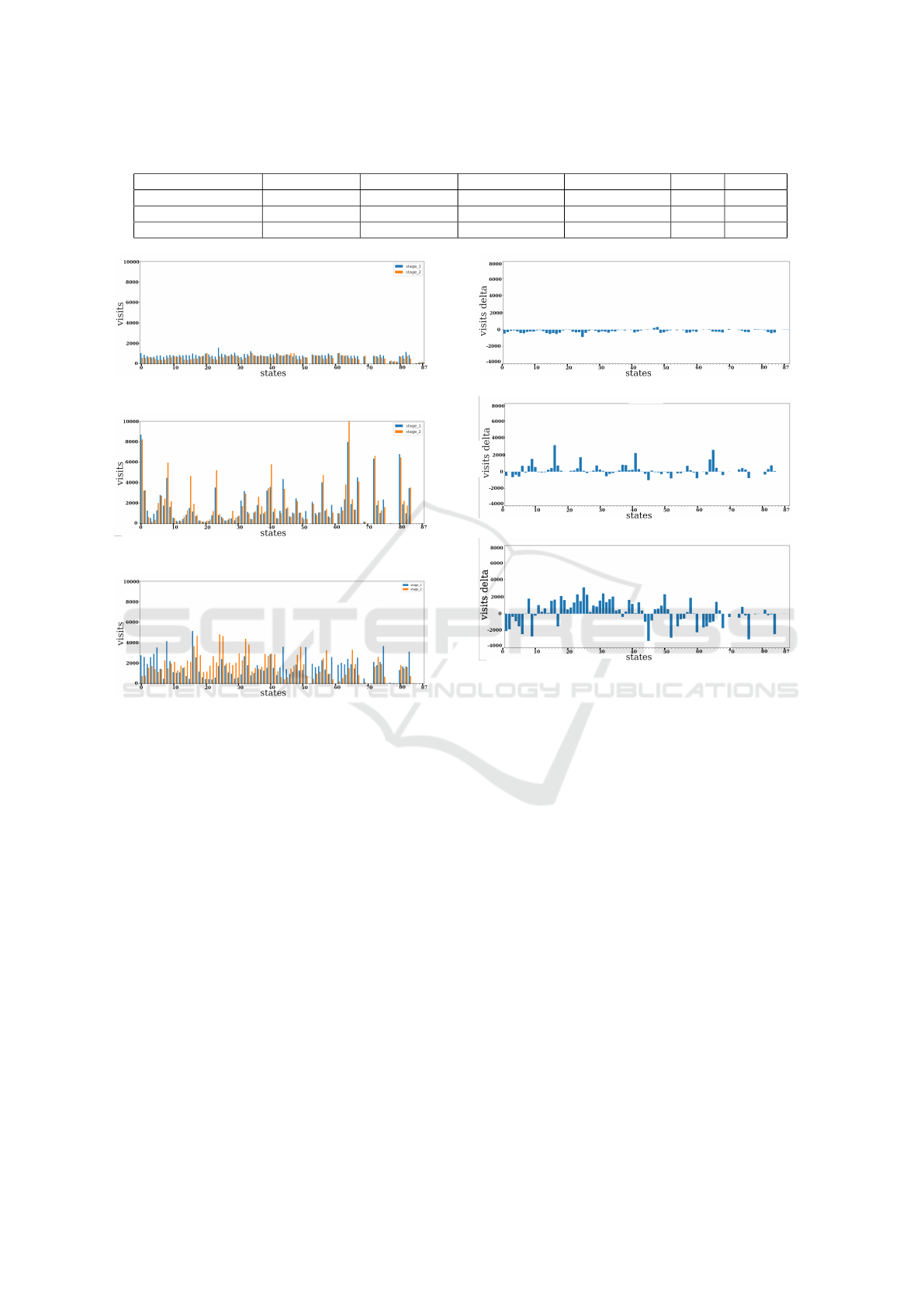
Table 2: Top 5 state visits in all 4 life stages. Union and intersection of the last two life stages.

Fist life stage Second life stage Third life stage Forth life stage Union LS3 ∩ LS4

Frontier 24, 34, 0, 20, 42 24, 62, 82, 53, 55 47, 46, 62, 45, 44 34, 61, 20, 42, 46 14 1

SOM(−quant

) 44, 0, 32, 59, 51 44, 0, 32, 59, 75 83, 0, 59, 32, 67 67, 0, 59, 32, 44 8 3

SOM(−quant

)+Frontier 44, 32, 81, 51, 6 51, 5, 44, 59, 6 51, 50, 59, 14, 44 13, 4, 12, 57, 51 13 1

(a) IM: Frontier method.

(b) IM: SOM(−quantization

error

) + Frontier.

Figure 3: Double bar ﬁgures.State Visits for two life stages

for an average of all 20 runs. Blue bars show the ﬁrst life

stage and the orange bars show the second life stage.

agent’s behaviour in these two periods and observe

how it changes as it progresses in its lifetime. Figure

3 depicts a comparison between the initial and ﬁnal

stages of different agents with different motivations.

The bars are colour-coded, with blue representing the

initial stage and orange representing the ﬁnal stage.

The Frontier method encourages the agent to priori-

tize states where it believes there is more to ﬁnd, pro-

moting exploration within the environment. As seen

in Figure3a, we observe that the Frontier method mo-

tivates the agent to explore all the states in a relatively

uniform way. No signiﬁcant difference in state vis-

its among various states is observed, as can be seen

through the conﬁdence interval of values for both life

stages, equaling 64.1 and 55.0 for life stages 1 and

2 respectively, within 95% conﬁdence. Also, we can

see that the range of state visits is smaller than the

other experiments, which means a better understand-

(a) IM: Frontier method.

(b) IM: SOM(−quant

Figure 4: State Visits for two life stages. Delta between

initial and ﬁnal life stages of states for each IM algorithm.

ing of the environment, efﬁcient navigation, more fre-

quent discovery of gateway states, and faster game

completion. Additionally, we observe that there is a

minimal number of visits to the ﬁnal states, which

is a count of zero in the other methods. This fact

highlights the Frontier agent’s superior navigation and

learning capabilities compared to other methods. The

next experiment for SOM quant

, feeds the value of

quant

counted by SOM as an intrinsical reward to

the agent. This approach leads the agent to be in-

trinsically rewarded for the states with lower quant

which are exactly the areas where SOM demonstrates

greater accuracy in clustering, whether they’re close

to the cluster centres or situated far from the bound-

aries. Notably, certain states exhibit higher visita-

tion counts in Figure 3a; many of these states are

visited more frequently during the latter half of their

life stages (indicated by a higher proportion of orange

colour compared to blue). This suggests that these

states represent the centroids of the clusters, exhibit-

ing minimal quant

NCTA 2023 - 15th International Conference on Neural Computation Theory and Applications

510

Finally, Figure 3c demonstrates combining the

Frontier motivation with quant

and we can see the

combination of characters of both other methods. The

centroid values are not extremely high and the explo-

ration seems more uniform. The results in this ﬁgure

highlight the effectiveness of the Frontier method in

promoting exploration in all other methods presented

in this study.

Next, we aim to analyze the behaviour of the agent

across two distinct life stages. Hence, we have com-

puted the delta between the ﬁnal and initial life stages

(Stage2 − Stage1) and visualized the results in Fig-

ure 4. Interpreting Figure 4, there are different per-

spectives to consider: If Stage2 > Stage1, it signiﬁes

that the agent visited states more often in its second

life stage, as shown by the positive value, suggesting

increased interest in these states during this period.

Conversely, if Stage2 < Stage1, the negative value in-

dicates that states were more frequently visited in the

ﬁrst half of the agent’s life, with reduced motivation

to revisit them in the second half.

This Figure further supports the observation high-

lighted in the previous bar charts, indicating that the

Frontier method promotes increased exploration by

the agent. The Delta bar in Figure 4a corresponds

to the Frontier method, exhibiting a relatively narrow

range of values compared to the other experiments,

indicating that the difference between the second and

ﬁrst life stages for each state is more consistent and

closer together. This proves the fact that the Frontier

method is explored in a more uniform way. Addi-

tionally, the predominantly negative delta values sug-

gest that the agent is visiting the states less in its sec-

ond life stage, which means it learned and understand

the states better. The next Figure 4b also proves the

behaviour of the SOM error agent we have seen in

Figure 4. We can see that the agent tends to visit

some states more in the second life stage resulting in

a greater positive value corresponding to the centroids

of the clusters. The last experiment which is the com-

bination of two methods, can be seen in 4c.

Graph Visualization for Agent’s Life Stages. In

this section, we aim to present the visualizations of

our state-transition graphs for our three different mo-

tivations. To understand the graphs better we have

presented the delta of the ﬁrst and second life stages

for each graph. By calculating the difference in state

visitation between these two stages (Stage2− Stage1)

, we recorded and visualized the visitation changes on

the graphs.

In the Frontier method Graph 5a, the sizes of

the nodes are mostly similar and smaller than the

other methods which shows the difference between

(a) IM: Frotier method.

(b) IM: Frontier +SOM(−quant

)

Figure 5: Graph representations for proposed methods.

the agent’s ﬁrst and second lifespans is smaller. These

ﬁndings align with the results discussed in the pre-

vious section, where we established that the Frontier

method enables the agent to navigate more uniformly

and learn better than the other methods. In the graph

generated from SOM with the −quant

technique (see

Figure 5c), we observe that certain states are larger in

size, indicating that the agent tends to visit them more

frequently during the second life stage. This pattern

corresponds to the centroids of the clusters formed by

the SOM algorithm. (We have inverted the graph for

better comparison with the other two experiments.)

The last experiment, as depicted in Graph 5b,

combines the characteristics of the two previous ex-

periments: SOM(−quant

) and Frontier. The agent

not only visits certain states more frequently, as seen

in the SOM experiment, but it also explores other

states beyond just the centroids of clusters, which is

a characteristic of the Frontier method. This combi-

nation of strategies allows the agent to have a more

Using Abstraction Graphs to Promote Exploration in Curiosity-Inspired Intrinsic Motivation

511

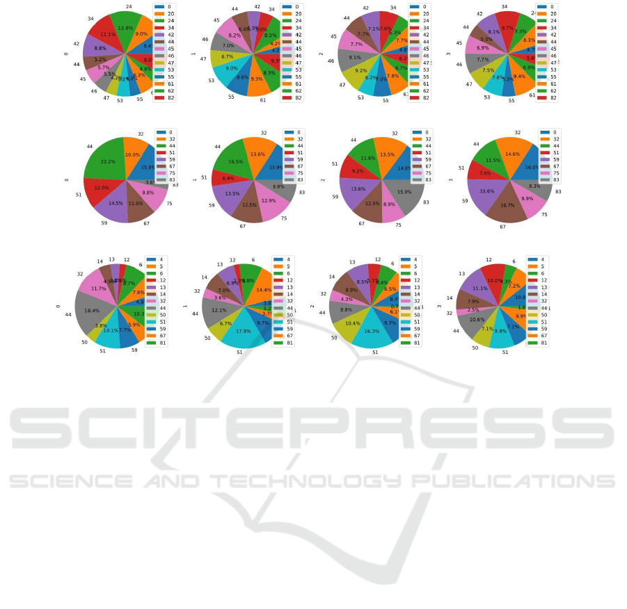
(a) IM algorithm: Frontier.

(b) IM algorithm: SOM (−quant

) + Frontier.

Figure 6: Top 5 steps visits of all life stages.

balanced exploration pattern, considering both moti-

vation methods.

Analysis of Key States in Different Stages of the

Agent’s Life. In this section, we divide our agents’

life stages into four equal parts and study how im-

portant nodes evolve in each phase. We consider the

most frequently visited node as the most important.

To illustrate the agent’s visits to the other top states in

different life stages, Figure 6 presents the results for

the top 5 states across all four stages together. More-

over, to gain a deeper understanding of the changes

occurring in the nodes, we present a table (2) listing

the top ﬁve states with the highest visitation counts

for each life stage.

Figure 6a, representing the Frontier method,

demonstrates a larger total number of states when

considering the top 5 states for each life stage. Addi-

tionally, by referring to Table 2, it becomes apparent

that the Frontier method exhibits a higher count in the

union of the top 5 visited states across all episodes.

These observations indicate that the Frontier method

explores more and accumulates a greater number of

state visits compared to other methods.

Figure 6b showing the SOM(−quant

) motivation

method, demonstrates reduced navigation, indicating

a tendency to focus on visiting clusters. This obser-

vation is further supported by examining Table 2 for

the same method, where the number of unions is 8,

representing the minimum count among the unions of

other methods.

By combining the two methods we can see the

agent is choosing fewer states in total to visit which

can be deﬁned as a medium behaviour between catch-

ing speciﬁc clusters and exploring more. Figure 6c

and Table 2 also support this fact by showing more

exploration than the SOM error method and less count

of state visits.

As we can see, the agent is exploring more in the

ﬁrst episodes to learn more.

5 CONCLUSION AND FUTURE

WORKS

This paper has proposed a method to incrementally

build a graph representation of the agents environ-

ment, and use this graph to analyse the behaviours

of different IM agents. We examined this approach

in a simulated computer game environment and com-

pared it to the SOM IM model. Based on our ﬁndings,

our proposed Frontier method demonstrates a higher

tendency towards exploration of all aspects of the en-

vironment in a relatively uniform manner.SOM error

algorithm demonstrates that the agent prefers to visit

states which are typically closer to the centroids of the

NCTA 2023 - 15th International Conference on Neural Computation Theory and Applications

512

clusters generated by the SOM. And lastly, the combi-

nation of the Frontier method with SOM yields a more

subtle behaviour in terms of clustering. This trans-

lates to a better understanding of the environment and

an accelerated process of ﬁnalizing the game.

Future work could employ graph representation to

uncover diverse agent behaviours by extracting more

graph data, such as cycle counts or frequently visited

paths, for better competence understanding. It can

also be applied to hierarchical RL to monitor skills

and behaviours across different levels.

REFERENCES

Aubret, A., Matignon, L., and Hassas, S. (2021). Elsim:

End-to-end learning of reusable skills through intrin-

sic motivation. In Machine Learning and Knowl-

edge Discovery in Databases: European Confer-

ence, ECML PKDD 2020, Ghent, Belgium, September

14–18, 2020, Proceedings, Part II, pages 541–556.

Springer.

Baraldi, A., Alpaydm, E., and Simpliﬁed, A. (1998). a new

class of art algorithms. International Computer Sci-

ence Institute, Berkley, CA.

Bellemare, M., Srinivasan, S., Ostrovski, G., Schaul, T.,

Saxton, D., and Munos, R. (2016). Unifying count-

based exploration and intrinsic motivation. Advances

in neural information processing systems, 29.

Buabin, E. (2013). Understanding reinforcement learning

theory for operations research and management. In

Graph Theory for Operations Research and Manage-

ment: Applications in Industrial Engineering, pages

295–312. IGI Global.

Clements, W. R., Van Delft, B., Robaglia, B.-M., Slaoui,

R. B., and Toth, S. (2019). Estimating risk and uncer-

tainty in deep reinforcement learning. arXiv preprint

arXiv:1905.09638.

Din, F. S. and Caleo, J. (2000). Playing computer games

versus better learning.

Eysenbach, B., Salakhutdinov, R. R., and Levine, S. (2019).

Search on the replay buffer: Bridging planning and

reinforcement learning. Advances in Neural Informa-

tion Processing Systems, 32.

Fritzke, B. (1995). A growing neural gas network learns

topologies, vol. 7.

Grossberg, S. (1976). Adaptive pattern classiﬁcation and

universal recoding: I. parallel development and cod-

ing of neural feature detectors. Biological cybernetics,

23(3):121–134.

Huang, Z., Liu, F., and Su, H. (2019). Mapping state space

using landmarks for universal goal reaching. Ad-

vances in Neural Information Processing Systems, 32.

Jin, J., Zhou, S., Zhang, W., He, T., Yu, Y., and Fakoor, R.

(2021). Graph-enhanced exploration for goal-oriented

reinforcement learning. In International Conference

on Learning Representations.

Kohonen, T. (2012). Self-organization and associative

memory, volume 8. Springer Science & Business Me-

dia.

Marsland, S., Nehmzow, U., and Shapiro, J. (2005). On-

line novelty detection for autonomous mobile robots.

Robotics and Autonomous Systems, 51(2-3):191–206.

Merrick, K. E. and Maher, M. L. (2009). Motivated rein-

forcement learning: curious characters for multiuser

games. Springer Science & Business Media.

Pathak, D., Agrawal, P., Efros, A. A., and Darrell, T. (2017).

Curiosity-driven exploration by self-supervised pre-

diction. In International conference on machine learn-

ing, pages 2778–2787. PMLR.

Peng, X. B., Chang, M., Zhang, G., Abbeel, P., and Levine,

S. (2019). Mcp: Learning composable hierarchi-

cal control with multiplicative compositional policies.

arXiv preprint arXiv:1905.09808.

Skupin, A., Biberstine, J. R., and B

orner, K. (2013). Visu-

alizing the topical structure of the medical sciences: a

self-organizing map approach. PloS one, 8(3):e58779.

Sutton, R. S. and Barto, A. G. (1998). Reinforcement

learning: an introduction mit press. Cambridge, MA,

22447.

Tu, L. A. (2019). Improving feature map quality of som

based on adjusting the neighborhood function. In Al-

musaed, A., Almssad, A., and Hong, L. T., editors,

Sustainability in Urban Planning and Design, chap-

ter 5. IntechOpen, Rijeka.

Using Abstraction Graphs to Promote Exploration in Curiosity-Inspired Intrinsic Motivation

513