An Observer Design Method Using Ultra-Local Model for Autonomous

Vehicles

Daniel Fenyes

1 a

, Tamas Hegedus

, Vu Van Tan

and Peter Gaspar

1,3

Institute for Computer Science and Control (SZTAKI), E

otv

os Lor

and Research Network (ELKH),

Kende u. 13-17, H-1111 Budapest, Hungary

Department of Automotive Mechanical Engineering, Faculty of Mechanical Engineering,

University of Transport and Communications, 3 Cau Giay Street, 100000 Hanoi, Vietnam

Department of Control for Transportation and Vehicle Systems, Budapest University of Technology and Economics,

Stoczek u. 2, H-1111 Budapest, Hungary

Keywords:

Observer, Model-Free Control, Ultra-Local Model, Lateral Velocity, Autonomous Vehicles.

Abstract:

The paper presents a novel observer design algorithm for autonomous vehicles. The technique is based on

the combination of a classical linear observer and the ultra-local model. The linear observer is easy to design

and it requires only a linear model of the considered system. However, it performs poorly when the linear

system cannot cover the system’s dynamics due to nonlinearities or unmodelled dynamics. The ultra-local

model aims to compensate for the nonlinear effects and improve the overall performances of the observer.

The proposed method is applied to a vehicle-oriented estimation problem: lateral velocity. The operation and

the effectiveness of the presented algorithm is demonstrated through several test scenarios in CarSim and also

using real-test measurements.

1 INTRODUCTION AND

MOTIVATION

The biggest challenges of the automotive industry are

related to the development of highly automated, au-

tonomous vehicles. Safe and reliable operation in ev-

ery possible trafﬁc situation is a prerequisite for the

widespread of fully autonomous vehicles. The algo-

rithm, which is responsible for vehicle control, con-

tains several layers such as sensing, decision-making,

and trajectory tracking. To guarantee the stable mo-

tion of the vehicle, the control systems require the

continuous measurement of several states of the car

such as velocities, angular velocities, and positions.

Some of these signals can be well-measured using

conventional onboard systems e.g. the angular veloc-

ities. However, other states are not directly measur-

able, e.g. lateral velocity. The estimation of the lat-

eral velocity of the vehicle is a common problem, for

which several solutions have been developed in the

past decades. These solutions can be divided into two

main groups:

• Model-based algorithms, which rely on mathe-

https://orcid.org/0000-0002-6143-5599

matical formulation of the vehicle dynamics.

• Non-model-based algorithms, which do not re-

quire a model but need a lot of training data of the

vehicle dynamics, e.g. machine learning-based

solutions.

One of the most common approaches to estimate

the lateral velocity of the vehicle is Kalman ﬁltering

method. This technique combines several measure-

ments from different sensors such as GPS and IMU

with a kinematic model of the vehicle, see (Chu et al.,

2010). The original Kalman ﬁlter can solely han-

dle linear models, which results in conservative solu-

tions. However, the extended Kalman ﬁlter is able to

deal with nonlinear models using linearization meth-

ods around operating points of the system, see (Huang

et al., 2017) . Although these solutions have already

been successfully applied to the estimation problem,

they have serious drawbacks. Since Kalman-ﬁlter-

based methods rely on accurate GPS signals, signal

loss, which may occur, signiﬁcantly reduces their per-

formance level.

Other model-based approaches use the classi-

cal observation technique such quadratic optimiza-

tion method (LQ) or polytopic modeling framework

(LPV). To apply these techniques the considered sys-

Fenyes, D., Hegedus, T., Van Tan, V. and Gaspar, P.

An Observer Design Method Using Ultra-Local Model for Autonomous Vehicles.

DOI: 10.5220/0012184300003543

In Proceedings of the 20th International Conference on Informatics in Control, Automation and Robotics (ICINCO 2023) - Volume 2, pages 41-49

ISBN: 978-989-758-670-5; ISSN: 2184-2809

tem must be observable, which means that certain

states of the system must be measurable.

LQ approach requires a linear model of the sys-

tem, which is convenient in terms of the design pro-

cess. But in the case of highly nonlinear systems, they

provide less accurate estimations. LPV framework al-

lows integrating a set of linear models to cover the

whole nonlinear dynamics of the considered system,

see (Kang et al., 2018),(Breschi et al., 2020). The

advantages of the model-based methods include that

they can provide theoretical guarantees. However, the

efﬁciency and accuracy of these methods are signif-

icantly inﬂuenced by the modeling process and the

accuracy of the yielded mathematical model. In addi-

tion, the effects of changing parameters must be taken

into account to avoid performance degradation.

The second group of methods consists of solu-

tions, which do not require a nominal model of the

system, such as machine learning-based, and data-

based approaches. In (Du et al., 2010) a neural

network-based solution is presented for estimating the

side-slip of the vehicle. Pace regression can also

be used to determine the side-slip angle as proposed

in (Fenyes et al., 2018). The advantage of these

solutions is that the lack of the modeling process

makes the design process easier, and also the non-

linear and uncertain effects can be handled more ef-

ﬁciently. However, these methods cannot provide

stability guarantees, which are essential for safety-

critical applications. There are other solutions, which

aim to combine the classical and non-model-based ap-

proaches to eliminate their individual drawbacks. For

example, in (Zhang et al., 2021) a method is proposed,

which uses a Kalman ﬁlter and a neural network to

compensate the effect of the possible GPS signal loss.

During the last decade, a new tool came up to ef-

ﬁciently solve modeling-related problems, called the

ultra-local model-based approach (Fliess and Join,

2013). The motivation behind the original structure

is to approximate the system in the given operating

point. This means that the nonlinearities and uncer-

tainties can be handled using the ultra-local model.

However, the original concept has been proposed for

a control system, and several works have been pub-

lished in the ﬁeld of observer design. In (Al Younes

et al., 2015) a nonlinear observer method is proposed

for aerial vehicles using the combination of the ultra-

local model-based technique and a Thau observer de-

sign.

This paper aims to combine a linear observer de-

sign method for lateral velocity estimation with the

results of the ultra-local model-based approach using

real test datasets. The original structure is modiﬁed

to take into account a priori knowledge of the system.

The modiﬁed structure is called the error-based ultra-

local model (Heged

us et al., 2022). Then, the whole

design process is carried out for a vehicle model with

a nominal parameter set. The advantage of the com-

bined solution is that by using the ultra-local model-

based part of the algorithm, the differences between

the nominal model and the real system can be han-

dled effectively. The proposed algorithm is tested on

real measurement data with different test scenarios.

The test scenarios have been carried out on ZalaZone

proving ground using a Lexus RH450 test vehicle.

The paper is structured as follows: Section 2

presents the error-based ultra-local model and gives

a short introduction to LQ observer design, then de-

tails the combined design approach. In section 3, the

vehicle-oriented example is presented including the

main steps. The effectiveness of the proposed algo-

rithm is demonstrated in the vehicle simulation soft-

ware, CarSim and using real test measurements in

Section 4 . Finally, the conclusion of the paper is sum-

marized in Section 5.

2 OBSERVER DESIGN USING

ULTRA-LOCAL MODEL

2.1 Error-Based Ultra-Local Model

The core idea of the error-based ultra-local model is

to create two ultra-local models: First one is com-

puted from the measured signals, second one is de-

rived from reference signals. Then, the error-based

ultra-local model (∆

nom

) is calculated as the deviation

of two ultra-local models, see (Fenyes et al., 2022):

(ν)

= F + αu (1a)

(ν)

re f

= F

nom

+ αu

nom,re f

(1b)

(ν)

− y

(ν)

re f

| {z }

(ν)

= F − F

nom

| {z }

∆

nom

+αu − αu

nom,re f

| {z }

α ˜u

(1c)

(ν)

= ∆

nom

+ α ˜u (1d)

where F is the ultra local model, u control signal, y

measured output, ν order of derivative, α denotes a

free tuning parameter, y

re f

is the reference output sig-

nal, u

nom,re f

denotes the referene control input The

reference signal y

re f

and the corresponding reference

input signal, u

nom,re f

Finally, the additional control input ( ˜u), which

compensates the unmodelled dynamics of the system,

can be computed as:

˜u =

−∆

nom,est

, (2)

ICINCO 2023 - 20th International Conference on Informatics in Control, Automation and Robotics

2.2 Discrete Linear Quadratic Observer

Linear Quadratic Observer design is based on a dis-

crete state-space representation of the considered sys-

tem, which can be written, in general form, as:

x(k + 1) = Φx(k) + Γu(k) (3a)

y(k) = c

x(k) (3b)

where Φ, Γ, c

are state matrices, x is the state-vector,

y is the output of the system, u is the control input

while k denotes the time step. The estimated state-

vector is computed as:

ˆx(k + 1) = Φ ˆx(k) + L(c

x(k) − c

ˆx(k)) (4)

The goal of the observer design to minimize the error

between the estimated states ˆx and the real states x:

e = x − ˆx, |e| → min! (5)

The error system can be written as (Kang and Kim,

2020):

e(k + 1) = Φe(k) − L(c

x(k) − c

ˆx(k)) = (6)

= (Φ − Lc

)e(k) (7)

where L is the gain-vector, which contains the opti-

mized gains for the observer.

This gain-vector can be computed by minimizing

the following cost function:

J =

∞

∑

i=1

(i)Qz

(i) + z

(i)Rz

(i)) (8)

where z

= x − ˆx is the performance, which minimizes

the error between the real and estimated states, and

= L(y − ˆy) is the control signal for correcting the

estimated states while Q and R are weighting matri-

ces. The optimal gain vector (L ) can be computed by

the discrete time algebraic Ricatti equation, which can

be formed as:

ΦP + PΦ

− Pc

−1

cP + Q = 0 (9)

= Pc

−1

(10)

where P > 0.

3 VEHICLE-ORIENTED

APPLICATION

In the followings, the proposed observer design is pre-

sented for a vehicle-oriented estimation problem. The

observer design consists of the following main steps:

1. The determination of the nominal model.

2. Selection of the required derivative order (ν).

3. Computation of the nominal reference signals

nom,re f

re f

)

4. Tuning of the parameter α.

5. Design of LQ observer based on the nominal

model.

6. Finally, the estimated states can be computed

as: ˆx(k + 1) = Φ ˆx(k) + Γ(u(k) −∆(k))+ L(y(k) −

ˆy(k))

The structure of the observer algorithm is illustrated

in Figure 1.

System

Model

State observer

Error-based ultra-local model

Combined observer

Figure 1: The structure of the proposed observer.

3.1 Determination of the Nominal

Model

In this paper, the one-track bicycle model is used dur-

ing the modeling phase of the lateral vehicle dynamics

(Rajamani, 2005). The basic idea behind this model

is that the front and rear wheels are replaced by one

wheel each placed on the longitudinal axis of symme-

try of the vehicle. The state-space representation of

the model is given as:



¨y







−

−C

− v

−

−C

−





| {z }



˙y



| {z }

(11)

with c

= [0 1].

ψ denotes the yaw-rate and I

is the yaw-inertia of the

vehicle. Moreover, C

gives the cornering stiffness of

the tires of the front and rear axes and β is the side-

slip angle. Moreover, l

gives distance from the axes

to CoG (center of gravity) and v

is the actual longi-

tudinal velocity. The lateral position of the vehicle is

given by y, whilst δ is the road wheel angle.

Finally, the continuous state-space representation

transformed into a discrete one:

(k + 1) = Φ

(k) + Γ

(k), (12a)

(k) = c

(k), (12b)

An Observer Design Method Using Ultra-Local Model for Autonomous Vehicles

3.2 Selection of Derivative Order and

Computation of the Reference

Signal

The goal of the observer design is to estimate the

lateral velocity (v

). Since the ﬁrst derivative of the

lateral velocity is the lateral acceleration, which is a

directly measurable signal, ν is set to ν = 1. Note

that the measured lateral acceleration (a

) has an ad-

ditional component therefore it is computed as ˙v

− v

ψ. The reference signals (u

nom,re f

, y

re f

) can

be computed using a model predictive approach as

detailed in (F

enyes et al., 2022). Note that during the

simulation/measurements, the vehicle is controlled by

a simple PD controller. PD controller does not use

the lateral velocity (v

), therefore it does not interfere

with the proposed observer method.

3.3 Tuning the Parameter α

In the literature, there is no elaborate method to de-

termine the optimal value of α. The determination of

the tuning value is solved using an iterative algorithm.

As pointed out by (Polack et al., 2019), when α → ∞,

the effect of the ultra-local model decreases and, in

contrast, when α → 0, the ultra-local model becomes

the major factor of the system. The computational

process is based on a previously saved dataset, which

contains the estimated ˆv

and also the accurate value

of the lateral velocity. In order to reach high-level

performance not a constant α is used but it depends

on the longitudinal velocity v

, which is highly corre-

lated to the nonlinear behavior of the vehicle. There-

fore, the measured dataset Ω is sorted into subsets.

Let A

∈ R

nx5

, A

= {v

y,i

,δ

y,i

} denote a

measurement set, which includes the measured sig-

nals at a speciﬁc time step. The whole dataset consists

of these measurement sets: A

∈ Ω ∀i ∈ N

. Then,

the dataset is divided into subsets {ω

,ω

...ω

} ⊆ Ω.

A subset is determined by a speciﬁc range of longitu-

dinal velocity A

∈ ω

x,i

x,min, j

< v

x,i

< v

x,max, j

}

where v

x,min, j

and v

x,max, j

are the lower and upper

bounds of j

subset.

The following optimization process must be per-

formed for each subset to get a set of α(v

min

∑

i=1

y,i

− ˆv

y,i

)

, v

y,i

∈ ω

(13)

where j is the index of the subsets and n is the

number of elements in j

subset. ˆv

y,i

is computed

from the elements of A

The main steps of the iterative algorithm, which

must be performed for each subset, are the following:

1. Design a nominal observer using the nominal

model.

2. Set the value of α to a high value.

3. Using the nominal observer and the actual value

of α, evaluate the algorithm for a predeﬁned test

scenario.

4. Compute the value of the error between the refer-

ence value and the output of the system e

, where

n denotes the n

iteration step.

5. If e

≥ e

n−1

or n > N

max

, quit the iteration.

6. Decrease the value of α then jump to Step 3.

3.4 LQ Observer Design

The goal of the observer design to minimize the error

between the estimated and the measured lateral veloc-

ities:

e = x − ˆx, |e| → min! (14)

This performance can be guaranteed by appropriately

chosen weighting matrices. In case of lateral ve-

locity estimation, the matrices are chosen to Q =

diag(1000,10), R = 1.

4 VALIDATION OF THE

ALGORITHM

In this section, simulation results are presented to

show the efﬁciency and the operation of the proposed

observer design approach. Moreover, at the end of

this section, an additional example is presented based

on a real measurement dataset. The whole algo-

rithm has been implemented in MATLAB/Simulink

and CarSim environment. During the simulations, a

B-class passenger car is used, whose nominal param-

eter can found in Table 1. Note that, the longitudinal

velocity (v

) is ﬁxed to v

= 10m/s during the linear

quadratic observer design.

Table 1: Parameters of the test vehicle.

m 1223 (kg)

,lr 1.083, 1.257 (m)

2330 (kgm

)

123000, 110000 (N/rad)

10 (m/s)

In the followings, three simulations example are

presented. In the ﬁrst simulation, the vehicle is driven

along a track with varying longitudinal velocity and

two observer algorithms are used to estimate the lat-

eral velocity: the proposed method and the nominal

ICINCO 2023 - 20th International Conference on Informatics in Control, Automation and Robotics

LQ observer. In the second simulation, the friction

coefﬁcient of the tire-ground contact is decreased to

µ = 0.5, which aims to show the operation of the pro-

posed observer method under extraordinary circum-

stances. In the last simulation, the type of the vehicle

is changed, which means that the nominal model sig-

niﬁcantly differs from the real vehicle.

4.1 Results of Tuning α

The presented tuning algorithm is performed on a

set of previous simulation from the simulation soft-

ware, CarSim. The test scenarios include lane change

maneuvers with v

= {1 − 120}km/h, and sinusoidal

steering signals. The resulted α values for each sub-

set can be found in Figure 2. It has a progressive part

between v

= {1 − 80}km/h and it reaches a constant

value around v

= 120km/h.

0 20 40 60 80 100 120

(km/h)

100

150

200

250

300

350

Paramter (-)

Data points

fitted curve

Figure 2: Parameter α.

4.2 Comparison of the Observers Under

Standard Circumstances

In the ﬁrst simulation, the vehicle is driven along F1

track of Hungary, shown in Figure 3. The track con-

tains several sharp bends, where the lateral velocity

can reach a high value. Furthermore, the longitudinal

velocity of the vehicle varies as illustrated in Figure

4. The velocity proﬁle consists of two main parts:

the ﬁrst one is the rapid changing part t = {0 − 200}s

and a slow changing part t = {200 − 400s}s in or-

der to cover the whole operating range of the vehicle.

Moreover, the measured signals (a

ψ) are corrupted

with white noises, whose variances: σ

= 0.04 and

= 0.01.

Figure 5 shows the lateral acceleration of the vehi-

cle during the test scenario. It can be seen, that max-

imum of a

is around 8m/s

, which is close to the

physical limit of the vehicle. In ﬁgure 6 similar phe-

nomenon can be observed, the maximum of yaw-rate

is about 0.6rad/s. In summary, it can be concluded,

−600 −400 −200 0 200 400 600

−200

200

400

600

800

1000

1200

Coordiante X (m)

Coordinate Y (m)

Figure 3: Test track.

0 50 100 150 200 250 300 350 400

Time (s)

Longitudinal velocity (m/s)

Figure 4: Longitudinal velocity of the vehicle.

that the simulations cover the whole operating range

of the vehicle.

0 50 100 150 200 250 300 350 400

−10

−8

−6

−4

−2

Time (s)

Lateral acceleration (m/s

)

Figure 5: Lateral acceleration of the vehicle.

200 250 300 350 400

−0.8

−0.6

−0.4

−0.2

0.2

0.4

0.6

0.8

Time (s)

Yaw−rate (rad/s)

Figure 6: Yaw-rate of the vehicle.

An Observer Design Method Using Ultra-Local Model for Autonomous Vehicles

The estimated and the measured lateral velocities

are depicted in Figures 7,8. Note that, this signal

is shown without the applied sensor noises. In the

ﬁrst section of the simulation, both observers provide

good results, however in the second half, the nominal

LQ observer has a signiﬁcant error. At that section,

the longitudinal velocity exceeds the nominal value

= 10m/s) for a long period of time, therefore the

LQ observer cannot provide good result. However,

it can be seen, when the velocity close to the nom-

inal value (t = 300s) the observer provides accurate

results. In contrast, the combined observer algorithm

estimate the lateral velocity in the whole simulation

with low error.

0 50 100 150 200

−0.8

−0.6

−0.4

−0.2

0.2

0.4

0.6

0.8

Time (s)

Lateral velocity (m/s)

LQ+UL Model

CarSim

Original LQ

Figure 7: Estimated and measured lateral velocities t = {0−

200}s.

200 250 300 350 400

−0.8

−0.6

−0.4

−0.2

0.2

0.4

0.6

Time (s)

Lateral velocity (m/s)

LQ+UL Model

CarSim

Original LQ

Figure 8: Estimated and measured lateral velocities t = {0−

200}s.

The last ﬁgure demonstrates the control inputs

of the observer. The blue line illustrates the com-

puted error-based ultra-local model (∆

nom

) while the

red line is the steering angle provided by the simula-

tion software. In general, the ultra-local model has a

higher amplitude, which aims to compensate for the

unknown and unmodeled part of the system.

0 50 100 150 200 250 300 350 400

−0.25

−0.2

−0.15

−0.1

−0.05

0.05

0.1

0.15

0.2

0.25

Time (s)

Control inputs (rad)

UL Model

Steering angle by CarSim

Figure 9: Inputs of the observers.

4.3 Simulation with Low Adhesion

Coefﬁcient

In the second simulation, the adhesion coefﬁcient be-

tween the tire and ground changed to µ = 0.5. This

demonstrates a case when the vehicle travels on the

snowy ground. Figure 10 shows the lateral acceler-

ation during this test scenario. The maximum value

of a

decreases to a

= 4m/s

, which is caused by

the low µ surface. It can also be seen, that the vehi-

cle reaches that value several times during the simu-

lation, which means that the vehicle loses its motion

stability. The nominal, linear observer cannot cope

with this motion as illustrated in Figures 11,12. In

other cases, the observer still provides acceptable re-

sults. The combined observer, however, can deal with

this nonlinear dynamics of the vehicle, and its result

matches with the measured lateral velocity as shown

in Figures 11,12.

0 50 100 150 200 250 300 350 400

−5

−4

−3

−2

−1

Time (s)

Lateral acceleration (m/s

)

Figure 10: Lateral acceleration in case of low µ.

4.4 Simulation Using Different Vehicle

Parameters

In the last test scenario, a case is investigated, when

the designed observer is applied to a completely dif-

ferent vehicle. The goal of this simulation is to show

the robustness of the proposed observer method. The

selected vehicle is a D-class passenger car, whose pa-

ICINCO 2023 - 20th International Conference on Informatics in Control, Automation and Robotics

0 50 100 150 200

−1.5

−1

−0.5

0.5

1.5

Time (s)

Lateral velocity (m/s)

LQ + UL Model

CarSim

Original LQ

Figure 11: Estimated and measured lateral velocities t =

{0 − 200}s.

200 250 300 350 400

−1

−0.5

0.5

1.5

Time (s)

Lateral velocity (m/s)

LQ + UL Model

CarSim

Original LQ

Figure 12: Estimated and measured lateral velocities t =

{200 − 400}s.

rameters can be found in Table 2. The track of the

vehicle is also changed to Michigan Waterford race-

track.

Table 2: Parameters of D-class car.

m 2013 (kg)

,lr 1.24, 1.68 (m)

4230 (kgm

)

230000, 180000 (N/rad)

10 (m/s)

The lateral velocity of the vehicle is depicted in

Figure 13. In this case, the maximum value of a

about 8m/s

, which indicates that the vehicle reaches

its psychical limits in this scenario similarly to the

previous test scenarios.

The estimated and the measured lateral velocities

can be seen in Figure 14. As it can be seen, the

nominal observer estimates the lateral velocity with

a large error since the model parameters signiﬁcantly

differ from the real ones. However, the proposed ob-

server still works well despite a short section between

t = {30 − 35}s. Note that the tuning parameter α has

also not been retuned for this vehicle, which can be

the reason behind this phenomenon.

0 50 100 150 200

−10

−8

−6

−4

−2

Time (s)

Lateral acceleration (m/s

)

Figure 13: Lateral acceleration in case of D-class car.

0 50 100 150 200

−0.5

0.5

Time (s)

Lateral velocity (m/s)

LQ + UL Model

Reference

Original LQ

Figure 14: Estimated and measured lateral velocities in case

of D-class car.

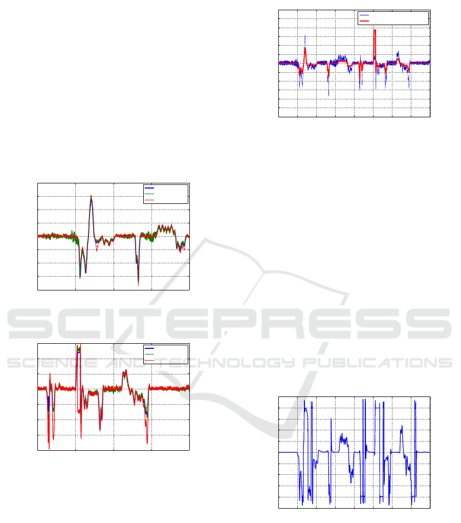
4.5 Example Using Real-Test

Measurements

To validate the performance of the proposed observer

algorithm, a 2km long test scenario has been per-

formed on the test ground using a Lexus RX450h test

vehicle. CarSim model is used to compare the results

of the observer and the measured data. This scenario

includes several bends, varying longitudinal velocity

with high acceleration and deceleration proﬁle. Fig-

ure 15 illustrates the longitudinal velocity of the vehi-

cle during the test. Its maximal value is about 25m/s

while the lowest value is 5m/s. Thus, the perfor-

mance of the observer can be tested in a wide range of

the vehicle dynamics. Figure 16 shows the measured

and the estimated lateral velocities. As the ﬁgure il-

lustrates, LQ-based observer provides poor results at

low and high longitudinal velocities. Whilst, the pro-

posed observer and CarSim’s model covers the mea-

sured lateral velocity well. The maximum of the error

is about 0.04m/s between 140 − 150s. In other cases,

the error is smaller than 0.02m/s.

Figure 17 demonstrates the lateral acceleration

during the test. The maximum of a

is almost 6m/s

which is high value for a SUV car. However, it does

not inﬂuence the accuracy of the estimation.

Figure 18 shows the two input signals: steering

angle and the output of the error-based ultra-local

An Observer Design Method Using Ultra-Local Model for Autonomous Vehicles

0 50 100 150

Time (s)

Longitudinal Velocity (m/s)

Measured

CarSim

Figure 15: Longitudinal velocities of the vehicle.

0 50 100 150

Time (s)

-0.8

-0.6

-0.4

-0.2

0.2

0.4

0.6

0.8

Lateral velocity (m/s)

CarSim

Proposed

LQ-based

Measured

Figure 16: Lateral velocities of the vehicle.

0 50 100 150

Time (s)

-6

-4

-2

Lateral acceleration (m/s

)

Figure 17: Lateral acceleration.

model. In this case, CarSim provides slightly worse

results compared to the previous test. The maxi-

mal deviation appears at low longitudinal velocity for

instance: 90 − 100s. The reason behind this phe-

nomenon could be that CarSim’s dynamical model is

ﬁtted for higher longitudinal velocities. In the reason-

able operating range, it ﬁts well the measurements.

0 50 100 150

Time (s)

-0.3

-0.2

-0.1

0.1

0.2

0.3

0.4

Inputs of the observer

F (-)

Steering angle (rad)

Figure 18: Control inputs.

5 CONCLUSION AND FUTURE

PLANS

In this paper, a novel combined observer design

method has been proposed using the linear quadratic

and the ultra-local model approaches. The LQ ob-

server was designed on a nominal model, which was

not expected to be accurate. The ultra-local model-

based part was able to approximate the unmodeled

dynamics of the system and to eliminate its effect,

which resulted in a more accurate estimation of the

observed state. The proposed observer design algo-

rithm has been implemented to a vehicle-oriented es-

timation problem: lateral velocity. The effectiveness

and the operation of the presented algorithm have

been demonstrated through simulation examples us-

ing CarSim and a real test measurement. The future

research directions include the investigation of co-

design with the Model-Free Controller and the analy-

sis of the closed-loop system.

ACKNOWLEDGEMENTS

The paper was funded by the National Research, De-

velopment and Innovation Ofﬁce under OTKA Grant

Agreement No. K 143599. The work of Daniel

Fenyes was supported by the Janos Bolyai Research

Scholarship of the Hungarian Academy of Sciences.

The research was partially supported by the European

Union within the framework of the National Labo-

ratoryfor Autonomous Systems (RRF-2.3.1-21-2022-

00002). The research was also supported by the Na-

tional Research, Development and Innovation Ofﬁce

through the project ”Cooperative emergency trajec-

tory design for connected autonomous vehicles” (NK-

FIH: 2019-2.1.12-T

ET VN).

ICINCO 2023 - 20th International Conference on Informatics in Control, Automation and Robotics

REFERENCES

Al Younes, Y., Noura, H., Muﬂehi, M., Rabhi, A., and

El Hajjaji, A. (2015). Model-free observer for state es-

timation applied to a quadrotor. In 2015 International

Conference on Unmanned Aircraft Systems (ICUAS),

pages 1378–1384.

Breschi, V., Formentin, S., Rallo, G., Corno, M., and

Savaresi, S. M. (2020). Vehicle sideslip estimation

via kernel-based lpv identiﬁcation: Theory and exper-

iments. Automatica, 122:109237.

Chu, L., Shi, Y., Zhang, Y., Liu, H., and Xu, M. (2010).

Vehicle lateral and longitudinal velocity estimation

based on adaptive kalman ﬁlter. In 2010 3rd Inter-

national Conference on Advanced Computer Theory

and Engineering(ICACTE), volume 3, pages V3–325–

V3–329.

Du, X., Sun, H., Qian, K., Li, Y., and Lu, L. (2010). A

prediction model for vehicle sideslip angle based on

neural network. In 2010 2nd IEEE International Con-

ference on Information and Financial Engineering,

pages 451–455.

enyes, D., Heged

us, T., N

emeth, B., Szabo, Z., and

asp

ar, P. (2022). Robust control design using ultra-

local model-based approach for vehicle-oriented con-

trol problems. In 2022 European Control Conference

(ECC), pages 1746–1751.

Fenyes, D., Hegedus, T., Nemeth, B., Szabo, Z., and Gas-

par, P. (2022). Combined lpv and ultra-local model-

based control design approach for autonomous vehi-

cles. In 2022 IEEE 61st Conference on Decision and

Control (CDC), pages 3303–3308.

Fenyes, D., Nemeth, B., Asszonyi, M., and Gaspar, P.

(2018). Side-slip angle estimation of autonomous road

vehicles based on big data analysis. In 26th Mediter-

ranean Conference on Control and Automation, pages

849–854.

Fliess, M. and Join, C. (2013). Model-free control. Inter-

national Journal of Control, 86(12):2228–2252.

Heged

us, T., F

enyes, D., N

emeth, B., Szab

o, Z., and

asp

ar, P. (2022). Design of model free control with

tuning method on ultra-local model for lateral vehicle

control purposes. pages 4101–4106.

Huang, Y., Bao, C., Wu, J., and Ma, Y. (2017). Estimation

of sideslip angle based on extended kalman ﬁlter. In

Journal of Electrical and Computer Engineering.

Kang, C. M. and Kim, W. (2020). Linear parameter vary-

ing observer for lane estimation using cylinder domain

in vehicles. IEEE Transactions on Intelligent Trans-

portation Systems, pages 1–10.

Kang, C. M., Lee, S.-H., and Chung, C. C. (2018). Discrete-

time lpv h

observer with nonlinear bounded varying

parameter and its application to the vehicle state ob-

server. IEEE Transactions on Industrial Electronics,

65(11):8768–8777.

Polack, P., Delprat, S., and d

Andr

ea Novel, B. (2019).

Brake and velocity model-free control on an actual ve-

hicle. Control Engineering Practice, 92:104072.

Rajamani, R. (2005). Vehicle dynamics and control.

Springer.

Zhang, B., Zhao, W., Zou, S., Zhang, H., and Luan, Z.

(2021). A reliable vehicle lateral velocity estimation

methodology based on sbi-lstm during gps-outage.

IEEE Sensors Journal, 21(14):15485–15495.

An Observer Design Method Using Ultra-Local Model for Autonomous Vehicles