Lateral Control for Automated Vehicles Based on Model Predictive
Control and Error-Based Ultra-Local Model
Tamas Hegedus
1 a
, Daniel Fenyes, Vu Van Tan
2
and Peter Gaspar
1,3
1
Institute for Computer Science and Control (SZTAKI), E
¨
otv
¨
os Lor
´
and Research Network (ELKH),
Kende u. 13-17, H-1111 Budapest, Hungary
2
Department of Automotive Mechanical Engineering, Faculty of Mechanical Engineering,
University of Transport and Communications, 3 Cau Giay Street, 100000 Hanoi, Vietnam
3
Department of Control for Transportation and Vehicle Systems, Budapest University of Technology and Economics,
Stoczek u. 2, H-1111 Budapest, Hungary
Keywords:
Ultra-Local Model, Lateral Control, Automated Vehicles.
Abstract:
The paper proposes a combined control design framework using Model Predictive Control (MPC) and ultra-
local model-based methods. The main idea behind the control algorithm is to exploit the advantage of both
approaches. During the control input computation, a simplified model is used, which has a significant impact
on the computational cost. Moreover, the simplified model does not contain hardly measurable or varying
vehicle-specific parameters, which makes the whole control design process easier. The ultra-local model is
used to deal with the unmodeled dynamics of the vehicle, by which the performance of the control system can
be increased. The effectiveness of the proposed control structure is demonstrated through trajectory tracking
problem of autonomous vehicles. The whole algorithm is implemented in a high-fidelity vehicle dynamics
simulation software, whose results are compared to an accurate model-based MPC in terms of computational
cost and tracking accuracy.
1 INTRODUCTION
In the last decades, several model-based control de-
sign techniques have been developed and successfully
implemented, such as PID, LQR, H
∞
(Batista et al.,
2019; Zhou and Doyle, 1998). However, for the ef-
fective application of these techniques, an accurate
model is essential, especially when high-performance
level must be guaranteed. One of the main difficulties
of the modeling process is that the parameters of the
system may change during its operation. Another is-
sue connected to accurate modeling of the system can
be challenging due to high nonlinearities and uncer-
tainties. On the other hand, an inaccurate model of
the system can lead to performance degradation, in-
stability, or constraint violation, which is not suitable
for safety-critical systems such as automated vehicles.
In addition to the mentioned control design meth-
ods, the Model Predictive Control (MPC) is a widely
used technique due to its advantages such as con-
straining specific state(s) of the system (Schwenzer
et al., 2021). The optimization-based control signal
a
https://orcid.org/0000-0001-8466-1102
calculation provides, for example, the possibility to
limit the input signal and guarantee constraints for
the given states of the system. Moreover, nonlinear-
ities and changing parameters can also be efficiently
taken into account during the control signal calcula-
tion (e.g., LTV-MPC, NMPC) (Allg
¨
ower et al., 2004;
Katriniok and Abel, 2011). However, this control de-
sign process still requires an accurate model or pa-
rameter estimation to provide high-performance level.
Another difficulty of the optimization-based methods
is that the complexity of the model and the length of
the control horizon have a high impact on the compu-
tational capacity.
In summary, simplifying the modeling process
or reducing the complexity of the model can make
the control design process easier. In order to avoid
the performances degradation caused by the simpli-
fied model, the ultra-local model-based approach can
be applied, which is also called in some literature
a Model-Free Control (MFC) structure (Fliess and
Join, 2013). The ultra-local model-based approach
has been successfully implemented for control de-
sign of many systems such as micro air vehicles
142
Hegedus, T., Fenyes, D., Van Tan, V. and Gaspar, P.
Lateral Control for Automated Vehicles Based on Model Predictive Control and Error-Based Ultra-Local Model.
DOI: 10.5220/0012184500003543
In Proceedings of the 20th International Conference on Informatics in Control, Automation and Robotics (ICINCO 2023) - Volume 2, pages 142-149
ISBN: 978-989-758-670-5; ISSN: 2184-2809
Copyright © 2023 by SCITEPRESS – Science and Technology Publications, Lda. Under CC license (CC BY-NC-ND 4.0)

(Barth et al., 2020) or active suspension (Ghazally I.
Y. Mustafa, 2019). However, this approach cannot
guarantee steady-state zero error. Therefore, a nomi-
nal feedback controller is applied, which is hard to ap-
propriately tune without a prior knowledge of the sys-
tem. Moreover, in (Wang and Wang, 2020) a hybrid
method is presented, with which both the advantages
of the ultra-local model and the MPC-based solution
can be exploited.
This approach can handle the parameter change
of the vehicle. The main advantage of the combined
structure is that it does not require an accurate model
of the system, which makes the whole control design
process easier. Furthermore, the parameters of a ve-
hicle may change during its operation, which can be
also effectively handled by the ultra-local model. An-
other aspect of this control structure, is that several
constraints can be applied to the states of the vehicle,
with which stable motion can be achieved. In addi-
tion, the computational time can be decreased using
the low-complexity model. In the paper, a kinematic
model-based solution is compared to another MPC al-
gorithm, which uses a dynamic, accurate model of the
vehicle. Finally, it is shown, that using the combined
solution, the same performance level can be reached
during the control of the vehicle. The simulations are
performed in high fidelity vehicle dynamics simula-
tion software, CarMaker.
The paper is structured as follows: The nominal
models are demonstrated, which are used during the
control of the vehicle in Section 2. Then, in Section 3
a description of the error-based ultra-local model can
be found. The MPC formalism can be found in Sec-
tion 4. The simulation example and the comparison
of the controllers are located in Section 5. Finally, the
whole paper and its contribution are summarized in
Section 6.
2 LATERAL MODELS OF THE
VEHICLE
In this section, two lateral models are presented for
the lateral modeling purposes of the vehicle. Firstly,
the two-wheeled bicycle model is described, while
the second model is created based on the kinematic
model of the system. The advantage of the first lateral
model is that it takes into account the dynamic effects
of the real vehicle. However, the second model has
less complexity and does not need dynamic parame-
ters of the controlled vehicle, which makes the mod-
eling process easier.
Dynamic Lateral Vehicle Model
In this subsection, the accurate lateral model is pre-
sented, which considers several effects of the dynam-
ics. For modeling purposes the two-wheeled lateral
vehicle model is used, which consists of the follow-
ing two main equations (Rajamani, 2005):
I
z
¨
ψ = α
f
C
f
l
f
− α
r
C
r
l
r
, (1a)
m( ¨y + v
x
˙
ψ) = α
f
C
f
+ α
r
C
r
, (1b)
where the side-slip of the front (α
f
) and rear
(α
r
) tires can be computed, using the lateral veloc-
ity (v
y
) and the yaw-rate (
˙
ψ) of the vehicle, as: α
f
=
δ −
v
y
+
˙
ψl
f
v
x
and α
r
=
−v
y
+
˙
ψl
r
v
x
. Moreover, m gives the
mass and the yaw inertia is given by I
z
. The distance
between the center of gravity and the axles is given
by l
f
and l
r
. The control input is the steering an-
gle of the vehicle (δ), while the longitudinal velocity
is expressed with v
x
. Based on the dynamical equa-
tions, the following state space representation can be
formed:
˙x
veh
= A
veh
(v
x
)x
veh
+ B
veh
(v
x
)δ, (2a)
A
veh
=



a
11
a
12
0 0
a
21
a
22
0 0
0 1 0 v
x
1 0 0 0



, B
veh
=



b
1
b
2
0
0



, (2b)
where a
11
= −
l
2
f
C
f
+l
2
r
C
r
I
z
v
x
, a
12
= −
l
f
C
f
−l
r
C
r
I
z
v
x
, a
21
=
−l
1
C
1
+l
2
C
2
mv
x
− v
x
, a
22
= −
C
f
+C
r
mv
x
, b
1
=
l
f
C
f
I
z
, and b
2
=
C
f
m
. The state vector is the following: x
veh
=
[
˙
ψ, v
y
, y
g
, ψ]
T
, which means the states of the system
are the yaw-rate, the lateral velocity of the vehicle in
the local coordinate system (v
y
), the global lateral po-
sition ( ˙y
g
= v
x
sin(ψ) + v
y
cos(ψ)), which is approxi-
mated for small yaw angles sin(ψ) ≈ ψ,cos(ψ) ≈ 1,
and the yaw-angle. The presented model is aug-
mented with the steering dynamics of the system,
in order to increase the performances of the control.
The steering system is modeled as a first-order term,
which can be written to the following state space rep-
resentation: A
st
= [
−1
T
st
], B
st
= [
1
T
st
], C
st
= [1]. In this
paper, the parameter of the steering system is set to
T
st
= 0.25, which is a reasonable value for the mod-
eling process. The state space representation model
of the system is augmented with the steering system,
which leads to the following matrices:
A
veh,st
=

A
st
0
1×4
B
veh
C
st
A
veh

, B
veh,st
=

B
st
0
4×1

,
C
veh,st
=

0
4×1
C
st

. (3)
Lateral Control for Automated Vehicles Based on Model Predictive Control and Error-Based Ultra-Local Model
143

The computation of the steering angle is per-
formed by an MPC method, which requires
discrete time model. Using (3) the discrete
model computed as: A
dyn
= e
A
veh,st
T
s
and B
dyn
=
(k+1)T
s
R
kT
s
e
A
veh,st
((k+1)T
s
−τ)
B
veh,st
τ, where T
s
is the sam-
pling time of the system, which is set to T
s
= 0.05s.
2.1 Kinematic Vehicle Model
After the description of the dynamic vehicle model,
the kinematic lateral model is detailed. The main
difference between this, and the previously described
model, is that many effects related to the vehicle dy-
namics are neglected during the modeling process
such as the tires, and the steering system. Moreover,
vehicle-specific parameters are not necessary for the
modeling process and the changing parameters also
do not need to consider. However, neglecting the dy-
namic effect may cause low performance or unstable
motion. During the MPC design, this model is ex-
tended with the effect of the error-based ultra-local
model to increase tracking performances. Two main
equations can be formulated for the lateral and angu-
lar motion of the vehicle (Lima et al., 2015):
dy
g
(t)
dt
= v
x
sinψ(t), (4a)
dψ(t)
dt
=
v
x
l
tanδ(t), (4b)
where the distance between the two axes is repre-
sented with l = l
f
+ l
r
. The longitudinal velocity can
be expressed as v
x
(t) = ds(t)/dt, with which (4) can
be transformed into space-domain as:
dy
g
(s)
ds
= v
x
sinψ(s), (5a)
dψ(s)
ds
=
δ(s)
l
. (5b)
The curvature of the trajectory (κ(s)) can be calcu-
lated using (5b) as κ(s) = δ(s)/l. One of the main
specifications for lateral control of a vehicle is related
to comfort requirement, which is fulfilled through
a smooth trajectory design. To meet this criterion,
the whole trajectory can be built up using clothoid
segments, which leads to the following expression:
κ(s) = κ
0
+ cs, where c provides the sharpness of the
given segment.
In the followings, the continuous equations are
transformed into discrete form, with the assumption,
that the vehicle travels with a constant velocity be-
tween two sampling time steps. Thus, the arc length
between two points can be computed as L
k
= v
x
(k)T
s
,
and using the clothoid segments, the curvature can be
formulated κ(k + 1) = κ(k) + c(k)L
k
. The lateral po-
sition and the yaw-angle of the vehicle can be also
transferred into discrete time:
ψ(k + 1) = ψ(k) + κ(k )L
k
+
1
2
c(k)L
2
k
, (6)
y
g
(k + 1) = y
g
(k) + L
k
sin(ψ(k)). (7)
Using the kinematic equation for the vehicle mo-
tion description, and assuming small angles, the
following discrete state-space representation can be
formed:
x
kin
(k + 1) = A
kin
x
kin
(k) + B
kin
c(k)


y
g
(k + 1)
ψ(k + 1)
κ(k + 1)


=


1 L
k
0
0 1 L
k
0 0 1


| {z }
A
kin


y
g
(k)
ψ(k)
κ(k)


+


0
L
2
k
2
L
k


|{z}
B
kin
c(k),
(8)
where the states (x
kin
(k)) are the lateral position, the
yaw-angle, and the curvature of the trajectory. More-
over, the control signal is the sharpness of the clothoid
segment. The output vector is computed as y
kin
(k) =
C
T
kin
x
kin
(k), C
T
kin
= [1, 0, 0].
During the computation of the ultra-local model-
based part of the control algorithm an additional con-
trol input, which is a steering angle in this paper, is
determined. However, in order to achieve the stable
motion of the vehicle, the effect of the additional con-
trol input is taken into account during the determina-
tion process of the bounds. In this paper, the effect
of the ultra-local-based part is considered through the
approximation of the lateral acceleration (a
y
), which
is limited during the optimization process. The lateral
acceleration is also approximated by a kinematic as-
sumption (Polack et al., 2017). The turning radius is
given as:
R =
l
tan(δ)
. (9)
The lateral acceleration is approximated as: a
y
=
v
2
R
.
Thus, the lateral acceleration at a given time step is
given by a
y
(k) = κ(k)v
2
(k). Moreover, the yaw-rate is
also can be approximated from the turning radius and
the actual longitudinal velocity
˙
ψ = v
x
/R. During the
computation of the lateral acceleration, the modeling
process of the steering system has been neglected.
ICINCO 2023 - 20th International Conference on Informatics in Control, Automation and Robotics
144

3 ERROR-BASED ULTRA-LOCAL
MODEL
This section describes the error-based ultra-local
model, which approximates the deviation between
the nominal model and the real system. Using this,
the non-modeled dynamics of the system can be also
taken into account and the performances of the con-
trol algorithm can be increased. For the computation
of the error-based ultra-local model, the ultra-local
model, and the nominal ultra-local model is needed.
The differences between them are considered as an
error-based ultra-local model (Heged
˝
us et al., 2023):
y
(ν)
= F + αu, (10a)
y
(ν)
re f
= F
nom
+ αu
nom
, (10b)
y
(ν)
− y
(ν)
r
| {z }
e
(ν)
= F − F
nom
| {z }
∆
+αu − αu
nom
| {z }
α ˜u
, (10c)
e
(ν)
= ∆ + α ˜u, (10d)
where F
nom
is the nominal ultra-local model, u
nom
is
the nominal control input of the system. Similarly
to the original structure, zero error can be achieved
only for the derivative of the error signal. This means,
that the augmented structure also requires a classical
controller for accurate tracking performances:
u = −
∆
α
− K (x, y
re f
). (11)
The main concept of the error-based ultra-local model
is introduced briefly in this paper, however, it is de-
tailed in (Heged
˝
us et al., 2023). In this case, the clas-
sical control algorithm K is chosen to an MPC, which
uses the actual states of the system (x) and also the
reference signal. The advantage of the MPC-based
extension is that this structure does not require addi-
tional signal computation such as the nominal control
input (u
nom
). During the design process, the nomi-
nal model of the system is used, which is described
in Subsection 2.1. The parameter α aims to scale the
derivative of the output to the control input. In this
paper, α is set to a constant value and it is selected to
α = 100. Moreover, for vehicle control-related prob-
lems, the value ν can be selected to ν = 2. More
details regarding the choice of the parameters can be
found in More details can be found in (Heged
˝
us et al.,
2022). Figure 1 shows briefly the combined control
structure of the control algorithm.
Vehicle
Error-based ultra
local model
Figure 1: The structure of the control algorithm.
4 LATERAL CONTROL DESIGN
The goal of the paper is to compare the performances
and computational capacity of the two different lat-
eral vehicle models. The nominal control algorithm is
selected for an MPC-based solution, with which sev-
eral constraints can be taken into account. The sta-
ble motion of the vehicle is guaranteed through these
constraints and also the effect of the additional con-
trol input can be taken into account. The goal during
the input signal calculation is to achieve the following
performances:
• The tracking error: y − y
re f
→ min!
• The interventions: δ → min!
In the followings, a brief introduction is presented
for the Model Predictive Control design.
4.1 Motion Prediction and the Cost
Function
In the first step, based on the system model and the
actual states of the vehicle, the states of the system
are predicted along the prediction horizon, which can
be made computed in a general form as:
y(k + 2) = C
T
(Ax(k + 1) + Bu(k + 1)) =
= C
T
(A(Ax(k) + Bu(k )) + Bu(k +1)),
(12)
where A,B,C
T
are the system matrices. In the second
step, the error between the actual output (y) and the
reference value (y
re f
) can be predicted as ε(k + i) =
y(k +i) −y
re f
(k +i). Using this, and the vector of the
reference values (R ), the error is computed for the
whole prediction horizon as:
Lateral Control for Automated Vehicles Based on Model Predictive Control and Error-Based Ultra-Local Model
145





ε(k + 1)
ε(k + 2)
.
.
.
ε(k + N
p
)




=





C
T
A
C
T
A
2
.
.
.
C
T
A
n





x(k) −




y
re f
(k + 1)
y
re f
(k + 2)
.
.
.
y
re f
(k + N p)




+





C
T
B 0 ··· 0
C
T
AB CB ··· 0
.
.
.
.
.
.
.
.
.
.
.
.
C
T
A
N
p
−1
B C
T
A
N
p
−2
B ··· C
T
B









u(k)
u(k + 1)
.
.
.
u(k + N
p
− 1)




= Ax(k) − R + BU
(13)
The goal is to define a cost function, with which
the optimization process is performed. Using (13) the
following function can be defined:
J(U) = (Ax(k) − R +BU)
T
Q(Ax(k) − R +BU)
+ UλU. (14)
where Q gives the weighting matrix, with which
the tracking performances can be influenced and the
intervention is weighted by λ. During the choice of
the weight values, the balance should be found be-
tween the accurate tracking and the energy consump-
tion (Camacho and Bordons, 2007). Using the cost
function (14), the following quadratic optimization
problem can be formed:
min
U
1
2
(U
T
γU + ω
T
U + U
T
α + ε), (15a)
such that
φU < b and l
b
≤ U ≤ l
u
, (15b)
where (15b) provides the constraints for the control
input, where l
b
gives the lower bound, while l
u
is the
upper bound. During the computation of the control
signal, constraints can be applied for the states of the
vehicle (b). Moreover, φ serves to select or compute
the constrained states of the system. Finally, γ, ω,α,ε
can be computed from (14) and the prediction horizon
is selected to N
p
= 30.
4.2 Constraints of the Vehicle
The additional control input (∆/α) has an impact on
the states of the vehicle, which can influence the sta-
ble motion. Therefore, constraints are defined for the
given states such as the yaw-rate, and lateral acceler-
ation to satisfy the stable motion requirements. How-
ever, taking into account the additional control input
is challenging since it cannot be considered directly
as a disturbance on the input signal, since it has im-
pact on the results of the optimization process and the
performances may be decreased. Thus, the additional
control input is built into the computation of the con-
straints during the optimization, with which the stable
motion of the vehicle is achieved.
On the other hand, the additional control input
cannot be computed for the whole optimization hori-
zon since measured signals of the system are also
needed. The idea to address this problem is to use the
computed value at the k
th
time step and to suppress
the value of the additional control input along the pre-
diction horizon. The prediction process is carried out
using the following expression:
G
pred
=
∆
α

1 −
1
T
2
∆
s
2
+ 2T
∆
s + 1

(16)
where T
∆
gives the time constant of the given lateral
dynamics of the vehicle, which can be determined by
the analysis of the dynamics see e.g. (Mondek and
Hrom
ˇ
c
´
ık, 2017). The additional control input predic-
tion is built up of two main parts. The first part is
the actual, computed ultra-local model (
∆
α
), while the
prediction is made using the transfer function (G
∆
),
which is a second-order term. In this paper, the time
constant is set to T
∆
= 0.2. The prediction process
of the additional control input is performed after the
discretization of G
∆
, which results in the matrices
A
∆
,B
∆
,C
∆
.
Since the formulation of the kinematic model does
not contain the lateral acceleration or the yaw-rate
of the vehicle, it is approximated by (9). Based on
(13), the predicted lateral acceleration can be formed
as a
y,p
= B(A
kin
,B
kin
,C
a
)U, where C
a
= [0, 0, v
2
x
]
T
.
Using the approximated lateral acceleration and the
predicted value of the additional control input, the
following constraints can be defined along the whole
prediction horizon:
a
y,p
+ E
∆
α

1 − B(A
∆
,B
∆
,C
∆
,U
∆
)

< b
ay
(17a)
a
y,p
− E
∆
α

1 − B(A
∆
,B
∆
,C
∆
,U
∆
)

> −b
ay
(17b)
where, E = v
2
/lE, and E = [1,1,...1]
T
, b
ay
∈
R
N
p
×1
gives the maximum lateral acceleration values.
B(A
∆
,B
∆
,C
∆
,U
∆
) can be computed as it is described
in (13) and the input (U
∆
) is the Heaviside step func-
tion. In this paper, the maximum value of the lat-
eral acceleration is set to |a
y,max
| = 7m/s
2
, with which
b
ay
= Ea
y,max
.
Furthermore, other states of the vehicle and the
maximum values of the steering angle are limited dur-
ing the optimization process. The constraints for the
yaw-rate of the vehicle are set to |
˙
ψ
max
| = 0.6rad/s.
Using the approximation
˙
ψ = v
x
/R and (17), the con-
straints can be determined for the yaw-rate value sim-
ICINCO 2023 - 20th International Conference on Informatics in Control, Automation and Robotics
146

ilarly to the lateral acceleration. The steering an-
gles are bounded (l
u
,l
b
) at 0.4rad. The maximum
lateral error is defined as: y
max,i
= y
re f ,i
+ R
i
and
y
min,i
= y
re f ,i
− R
i
. The R
i
is chosen in such a way,
that the first element (R
1
) of the R vector is the high-
est and the last value (R
N p
) is the lowest. Between the
two elements, the values decreased equidistantly, with
a step of d = (R
1
−R
N p
)/N p. The highest value is set
to R
1
= 0.6m and the lowest is R
N p
= 0.05m. Using
these constraints, the vector of the bounds (b) can be
created. Finally, φ is determined based on the appro-
priately chosen matrix C. These constraints serves to
guarantee the stable motion of the vehicle and applied
for both of the MPC controllers during the simula-
tions.
Structure and the Calculation of the
Derivatives
Finally, in Figure 2 the control structure is presented,
which contains the MPC with the kinematic model
and uses also the results of the error-based ultra-local
model. The MPC computes the input sequence for
the system. Using the first value of the input sig-
nal, the mathematical formulation of the system, and
the actual states, the output of the system can be ap-
proximated for the following time step (y
MPC
(k +2)).
Moreover, for the computation of the nominal ultra-
local model (10b), the derivative signals are also
needed, which is illustrated with D.A. in Figure 2. On
the other hand, the measurable signals, and the real in-
put of the system are used for the computational pro-
cess of the ultra-local model. The deviation between
these models gives the error-based ultra-local model,
which is an additional control input of the system. Fi-
nally, z
−1
aims to match between the input and the
output signals and between the two ultra-local mod-
els.
MPC with kinematic
model
Vehicle
D.A.
D.A.
-
+
-
+
-
+
-
+
Figure 2: Structure of the combined control algorithm.
It is described in (10), that the derivative of the
measured, and the approximated outputs are required.
The accelerations, which are equivalent to the 2
nd
derivative of the outputs, can be calculated as (Polack
et al., 2019):
a
y,est
= −
5!
2T
5
Z
T
0
(−T
2
+ 6T τ − 6τ
2
)y(τ)dτ (18)
where T > 0 must be chosen small and x(t) denotes
the longitudinal position of the vehicle and T gives
the time window of the filter. However, the pro-
posed equations cannot be implemented in practice.
Thus, the numerical solution is approximated using
the Simpson’s rule (Polack et al., 2019):
Z
b
a
f (x)dx ≈
b − a
90

7 f (a) + 32 f

a + b
4

+
+12 f

2(a + b)
4

+ 32 f

3(a + b)
4

+ 7 f (b)

(19)
During the implementation of the proposed algorithm
the output and the approximated output of the system
are derivated using (18), (19).
5 SIMULATION
In this section, the algorithm is tested on a vehicle dy-
namic simulation software, CarMaker. This section
aims to show the performances and the effectiveness
of the combined solution. Moreover, the control per-
formances using the different models are also com-
pared to each other. The following simulations are
performed:
• Kinematic model-based MPC with the error-
based ultra-local model
• MPC with the dynamic model of the vehicle
• Kinematic model-based MPC without the error-
based ultra-local model
During the simulations, the vehicle is selected to
a Tesla Model S. The accurate vehicle parameters can
be found in the simulation software, with which the
lateral model (3) can be tuned properly. On the other
hand, the kinematic lateral model does not require
hardly determinable vehicle-related parameters. The
whole algorithm is tested through trajectory tracking,
which is selected to a lane-change-like reference path.
The maximum lateral deviation of the lane changes
varies randomly, and also the velocity varies. In Fig-
ure 3 the measured velocity profile of the vehicle can
be seen.
Figure 4 presents the measured and the reference
lateral position of the vehicle. It can be concluded that
Lateral Control for Automated Vehicles Based on Model Predictive Control and Error-Based Ultra-Local Model
147

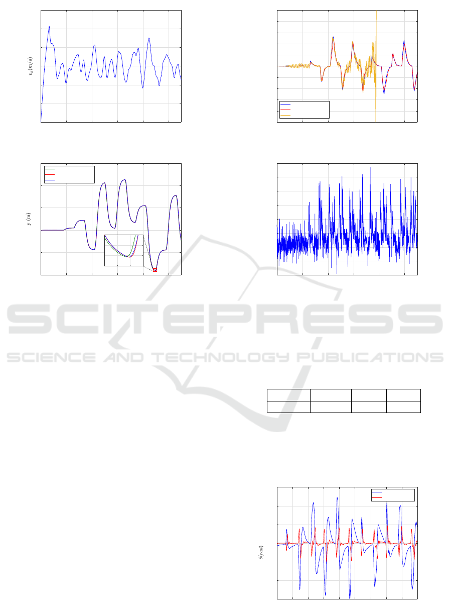
0 20 40 60 80 100
Simulation time (s)
10
15
20
25
30
35
40
Figure 3: Longitudinal velocity of the vehicle.
0 20 40 60 80 100
Simulation time (s)
-10
-5
0
5
10
15
Reference
Kinematic MPC + UL
Dynamical MPC
88 89 90 91
-9.2
-9
-8.8
-8.6
Figure 4: Lateral position of the vehicle.
both of the control algorithms can steer the vehicle
along the given reference trajectory accurately.
The kinematic MPC, with the error-based ultra-
local model, reaches the performances of the dynam-
ical MPC. In Figure 5 the computed lateral errors are
presented to make it easier to compare the control al-
gorithms. However, in this case, the results of the
kinematic MPC, without the additional control input,
are also demonstrated with the yellow line. It can be
examined that this algorithm cannot control the vehi-
cle along the given trajectory and it loses its stability.
Since the dynamical effects are not modeled and also
the steering system is neglected, an oscillation occurs
and finally the constraints cannot be met and the MPC
is not capable to compute a feasible solution with the
given limitations for the states.
Another important aspect is to compare the re-
sults in terms of computational capacity. The opti-
mization time saved for the same simulation case us-
ing the dynamical MPC (T
dyn,MPC
) and the kinematic
model-based MPC with the ultra-local model-based
part. Then the rate of the two algorithms is computed
as C
r
= T
dyn,MPC
/T
kin,MPC
. To eliminate external fac-
tors as much as possible, the same simulation case is
simulated 10 times and the results are averaged. The
results are shown in Figure 6.
Figure 6 depicts that the computational capacity
of the kinematic model-based MPC with the ultra-
0 20 40 60 80 100
Simulation time (s)
-0.5
-0.4
-0.3
-0.2
-0.1
0
0.1
0.2
0.3
0.4
0.5
Lateral error (m)
Kinematic MPC +UL
Dynamical MPC
Kinematic MPC
Figure 5: Lateral errors during the test scenarios.
0 20 40 60 80 100
Simulation time (s)
1.5
2
2.5
3
3.5
4
4.5
5
5.5
Computational time rate (-)
Figure 6: Rate of the computational capacities.
local model is much lower than the complex, dynamic
model-based MPC. In the worst case, it is 1.5 times
faster and the highest difference is more than 5x. In
the following table, the maximum, minimum, mean,
and standard deviation (Std.) of the rate of the com-
putational times are presented.
Highest Lowest Mean Std.
5.35 1.53 2.93 0.547
The computed steering angles can be seen in Fig-
ure 7. The blue line represents the results of the MPC,
and the red lines show the computed error-based ultra-
local model. Using these signals, the vehicle is driven
along the predefined lane-change maneuvers.
20 30 40 50 60 70 80 90 100 110
Simulation time (s)
-0.03
-0.02
-0.01
0
0.01
0.02
0.03
Kinematic MPC
Ultra-local model
Figure 7: Control inputs during the test scenarios.
ICINCO 2023 - 20th International Conference on Informatics in Control, Automation and Robotics
148

Finally, the lateral accelerations are presented. It
can be seen, the maximum value of the acceleration
reaches 3m/s
2
, which is an appropriate value for ev-
eryday traffic situations.
10 20 30 40 50 60 70 80 90 100 110
Simulation time (s)
-4
-3
-2
-1
0
1
2
3
4
Dynamical MPC
Kinematic MPC + UL
Figure 8: Lateral accelerations during the test scenarios.
6 CONCLUSIONS
The paper has presented a novel control design ap-
proach, which took the advantages of low computa-
tional cost MPC and error-based ultra-local model.
The proposed control algorithm was able to guarantee
a high-performance level and to take into account the
state constraints of the system. The efficiency and the
operation of the proposed method have been demon-
strated through a vehicle-oriented control problem,
trajectory tracking. The designed controller has been
compared to a high-computational cost MPC to show
the performance level of the presented algorithm. The
comparison has been carried out in the high-fidelity
simulation software, CarMaker.
ACKNOWLEDGEMENTS
The research was supported by the European Union
within the framework of the National Laboratory for
Autonomous Systems (RRF-2.3.1-21-2022-00002).
The paper was partially funded by the National Re-
search, Development and Innovation Office under
OTKA Grant Agreement No. K 143599. The research
was also supported by the National Research, De-
velopment and Innovation Office through the project
”Cooperative emergency trajectory design for con-
nected autonomous vehicles” (NKFIH: 2019-2.1.12-
T
´
ET VN).
REFERENCES
Allg
¨
ower, F., Findeisen, R., and Nagy, Z. (2004). Nonlinear
model predictive control: From theory to application.
Journal of The Chinese Institute of Chemical Engi-
neers, 35:299–315.
Barth, J. M., Condomines, J.-P., Bronz, M., Moschetta, J.-
M., Join, C., and Fliess, M. (2020). Model-free con-
trol algorithms for micro air vehicles with transition-
ing flight capabilities. International Journal of Micro
Air Vehicles, 12.
Batista, J. G., Souza, D. A., dos Reis, L. L., Filgueiras,
L. V., Ramos, K. M., Junior, A. B., and Correia, W. B.
(2019). Performance comparison between the PID
and LQR controllers applied to a robotic manipula-
tor joint. In IECON 2019 - 45th Annual Conference
of the IEEE Industrial Electronics Society, volume 1,
pages 479–484.
Camacho, E. F. and Bordons, C. (2007). Model predictive
control. Springer London.
Fliess, M. and Join, C. (2013). Model-free control. Inter-
national Journal of Control, 86(12):2228–2252.
Ghazally I. Y. Mustafa, Haoping Wang, Y. T. (2019).
Model-free adaptive fuzzy logic control for a half-car
active suspension system. Studies in Informatics and
Control, 28.
Heged
˝
us, T., F
´
enyes, D., N
´
emeth, B., Szab
´
o, Z., and
G
´
asp
´
ar, P. (2022). Design of model free control with
tuning method on ultra-local model for lateral vehicle
control purposes. pages 4101–4106.
Heged
˝
us, T., F
´
enyes, D., Szab
´
o, Z., N
´
emeth, B., Luk
´
acs,
L., Csikja, R., and G
´
asp
´
ar, P. (2023). Implementation
and design of ultra-local model-based control strategy
for autonomous vehicles. Vehicle System Dynamics,
0(0):1–24.
Katriniok, A. and Abel, D. (2011). LTV-MPC approach for
lateral vehicle guidance by front steering at the limits
of vehicle dynamics. In 2011 50th IEEE Conference
on Decision and Control and European Control Con-
ference, pages 6828–6833.
Lima, P. F., Trincavelli, M., Martensson, J., and Wahlberg,
B. (2015). Clothoid-based model predictive control
for autonomous driving. In 2015 European Control
Conference (ECC), pages 2983–2990.
Mondek, M. and Hrom
ˇ
c
´
ık, M. (2017). Linear analysis of
lateral vehicle dynamics. In 2017 21st International
Conference on Process Control (PC), pages 240–246.
Polack, P., Altch
´
e, F., d
´
Andr
´
ea Novel, B., and
de La Fortelle, A. (2017). The kinematic bicycle
model: A consistent model for planning feasible tra-
jectories for autonomous vehicles? 2017 IEEE Intel-
ligent Vehicles Symposium (IV), pages 812–818.
Polack, P., Delprat, S., and d
´
Andr
´
ea Novel, B. (2019).
Brake and velocity model-free control on an actual ve-
hicle. Control Engineering Practice, 92:104072.
Rajamani, R. (2005). Vehicle dynamics and control.
Springer.
Schwenzer, M., Ay, M., and Abel, D. (2021). Review on
model predictive control: an engineering perspective.
The International Journal of Advanced Manufactur-
ing Technology, 117:1327–1349.
Wang, Z. and Wang, J. (2020). Ultra-local model predictive
control: A model-free approach and its application on
automated vehicle trajectory tracking. Control Engi-
neering Practice, 101:104482.
Zhou, K. and Doyle, J. C. (1998). Essentials of Robust Con-
trol. Prentice-Hall.
Lateral Control for Automated Vehicles Based on Model Predictive Control and Error-Based Ultra-Local Model
149