Simultaneous Planning of the Path and Supports of a Walking Robot

Paula Mollá-Santamaría

, Adrián Peidró

, Arturo Gil

, Óscar Reinoso

1,2 d

and Luis Payá

Instituto de Investigación en Ingeniería de Elche (I3E), Universidad Miguel Hernández de Elche,

Avda. de la Universidad s/n, Edificio Innova, 03202 Elche, Alicante, Spain

ValgrAI: Valencian Graduate School and Research Network of Artificial Intelligence,

Camí de Vera s/n, Edificio 3Q, 46022 Valencia, Spain

Keywords: Path Planning, Support Planning, Stability, Non-Coplanar Contacts, Walking Robot.

Abstract: In this paper we study the simultaneous planning of the path and leg supports of an eight-legged robot on

uneven terrain. We use the A-star algorithm (A*), which searches for the shortest path between two points.

First, the terrain is modelled with a triangular mesh and the triangles are subdivided to take the centroids of

these triangles as the search space of the A*. Secondly, with respect to the original A*, the stability of the

robot at each centroid is considered, so that the cost at a centroid is penalised if the robot is unstable (i.e., the

robot slips and/or tips over), or the cost is zero if it is stable. The stability at each contact point is determined

by calculating that the ground reaction at that point is contained in a linear approximation of the friction cone.

Finally, the path, the contact points of each leg, as well as the robot's posture at each position are obtained.

1 INTRODUCTION

This paper presents a solution for the path planning of

an eight-legged modular robot in rough natural

terrains consisting of different slopes. We determine

the sequence of positions and orientations that the

robot must visit in order to move from an initial point

to a final point of the terrain, including the supports

or footholds where the robot must place all feet for

each position of the path, to guarantee stability, i.e.,

to prevent slipping and tipping over.

For legged robots moving on horizontal planes

with sufficient friction to prevent slippage, one of the

most extended stability tests is based on the Zero

Moment Point (ZMP) (Vukobratović and Borovac,

2004), which is the point respect to which contact

moments have no horizontal components. If the ZMP

belongs to the convex hull of the support points, the

robot will not tip over.

For robots with legs supported on different planes,

or when the ground cannot offer sufficient friction to

neglect slippage, the ZMP test is insufficient and the

https://orcid.org/0009-0003-5447-0278

https://orcid.org/0000-0002-4565-496X

https://orcid.org/0000-0001-7811-8955

https://orcid.org/0000-0002-1065-8944

https://orcid.org/0000-0002-3045-4316

Contact Wrench Cone (CWC) (Hirukawa et al., 2006)

should be studied instead. The CWC is based on the

idea that, for each point of contact of the robot with

the ground, there is a reaction force from the ground

that should be inside a friction cone whose axis is

normal to the ground and whose aperture depends on

the coefficient of friction. For computational

efficiency, such friction cones are approximated by

inscribed pyramids. The vectors 𝐟



along the lateral

edges of these pyramids, together with their moments,

constitute a set of 6-dimensional wrenches that,

counted for all contact points of the robot, span the 6-

dimensional Contact Wrench Cone. If the net wrench

acting on the robot due to inertia, gravity and external

forces (excluding reactions from the ground) belongs

to the CWC, the robot will not tip over or slip.

The CWC has been widely used to plan the

dynamically stable locomotion of legged robots, both

bipedal humanoids (Dai y Tedrake, 2016; Navaneeth,

Sudheer, and Joy, 2022) and quadrupedal (Aceituno-

Cabezas et al., 2017). Most papers depart from a

precomputed set of footholds along the terrain, at

648

Mollá-Santamaría, P., Peidró, A., Gil, A., Reinoso, Ó. and Payá, L.

Simultaneous Planning of the Path and Supports of a Walking Robot.

DOI: 10.5220/0012184600003543

In Proceedings of the 20th International Conference on Informatics in Control, Automation and Robotics (ICINCO 2023) - Volume 1, pages 648-656

ISBN: 978-989-758-670-5; ISSN: 2184-2809

which the robot should support its legs during the

trajectory, and then they focus on solving the

trajectory of the center of mass to guarantee that

gravito-inertial wrenches are in the CWC within some

margin, while minimizing centroidal angular

momentum. Recent papers such as (Aceituno-

Cabezas et al., 2018) or (Jenelten, Grandia,

Farshidian, and Hutter, 2022) do not assume a

precomputed set of footholds, which are planned at

the same time that the global locomotion of the robot,

solving mixed-integer convex optimization problems

or using graduated optimization techniques. The

simultaneous planning of the path of the robot and of

the footholds yields more optimal and natural

solutions. Other remarkable works that use the CWC

are (Orsolino et al., 2018), where the CWC is

intersected with a polytope that considers limits on

actuation torques, or Ellenberg and Oh (2014), who

use the CWC to analyze the stability of humanoids

climbing ladders, taking into account limits on the

contact wrenches that the environment can provide.

Typically, the stability test based on the CWC is

computationally demanding, considering that it

requires many operations to first build a polytope that

is the convex hull of dozens of 6-dimensional contact

wrenches, and then check if the gravito-inertial

wrenches acting on the robot belong to this polytope.

Some papers have tried to reduce the cost of these

operations to check stability while controlling the

robot in real time. Li et al. (2022) present a simplified

test that approximates the contact polygon by an

effective segment, sacrificing accuracy for efficiency.

Caro and Kheddar (2016) change checking the 6D

polytope for checking if the centroidal acceleration

belongs to a 3D volume. Finally, Caron, Pham and

Nakamura (2017) project the CWC on a 2D polygon

to which the ZMP should belong to guarantee

stability, generalizing the notion of ZMP to situations

with insufficient friction or non-coplanary contacts.

In this paper, we present a solution for the

simultaneous planning of the path and supports of a

modular eight-legged robot described in Section 2,

which should explore natural terrains consisting of

planes with different orientations where slippage

cannot be neglected. First, in Section 3, we describe

the modeling of the terrain, which is approximated by

a triangular mesh. Next, in Section 4, we present the

stabilty test, which avoids building the 6-dimensional

CWC and instead solves iteratively a quadratic and

underdetermined system of equations using the

Newton-Raphson method, performing the stability

test roughly 10 times faster than by building the

CWC. Section 5 proposes our algorithm to

simultaneously plan the path and supports of the

legged robot, which is based on the A-star (A*)

algorithm, but incorporating instability as a penalty to

the cost function (among other sub-costs). Then,

Section 6 illustrates the developed algorithm by

means of examples. These examples demonstrate the

feasibility of the paths planned by the proposed

algorithm, comparing the results obtained when

considering stability or when ignoring it (in which

case, the robot would fall down steep inclines).

Finally, Section 7 summarizes the conclusions and

suggests future lines of research, which will be

mainly directed towards speeding up the proposed

method, so that it can be used in real time.

2 ROBOT DESCRIPTION

This section describes the modular walking robot

whose optimal path is planned in this paper, from an

initial to a final position in a rugged natural

environment, also determining the contact points on

the ground.

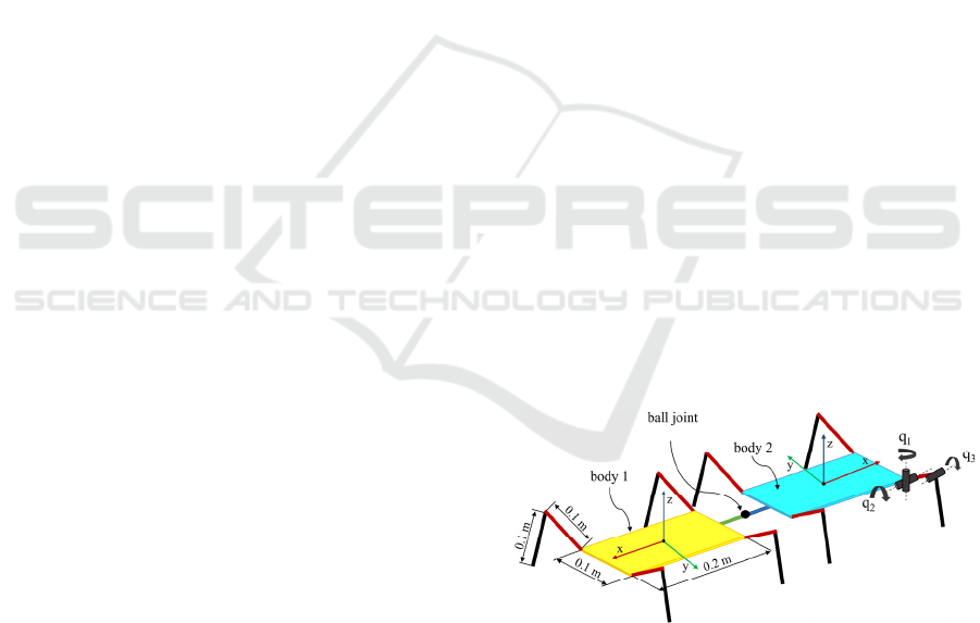
The robot presented in Figure 1 consists of two

identical modules connected by a spherical or ball

joint. The modules have a central body that can move

and orient itself in the x, y, and z axes and four legs

with three degrees of freedom each (q

, q

) that

allow it to move efficiently, where q

provides the

forward and backward movement of the leg, q

allows

the raising and lowering of the leg, and q

facilitates

the bending or stretching of the leg. Each module of

the robot has eighteen degrees of freedom, giving it

great freedom of movement for moving over rough

terrain.

Figure 1: Wireframe representation of the studied modular

legged robot.

3 TERRAIN MODELLING AND

SUBDIVISION

The planning of the robot's path and the determination

of the points of contact with the environment are the

objectives of this article. To this purpose, this section

Simultaneous Planning of the Path and Supports of a Walking Robot

649

describes the modelling and pre-processing of the

terrain on which the robot moves, considering that all

the robot's feet will be resting on the ground at each

position of the planned path.

The modelled terrain consists of several ramps

with different inclinations surrounding the

environment, requiring the robot to climb three ramps

to reach the highest point. It is important to note that

the initial terrain is defined by a triangular mesh in

STL format. To achieve this, we first used 3D design

software, specifically Autodesk Inventor, to create

the CAD model of the terrain. Then, we exported the

model in STL format, as this format is capable of

representing solid objects by approximating their

surface with triangles in a graphical manner. In real

scenarios, a point cloud of the environment may be

obtained using range sensors, and this point cloud

may be used as the starting point to model the terrain

in a similar way as described in this paper.

To undertake the planning of the robot's path, it is

necessary to start with a point cloud to identify the

nodes or points that will be part of the optimal path

from the initial to the final position. Since the terrain

is composed of triangles, the centroids of these

triangles are used as search points for the path. In

order to obtain a denser mesh of nodes and to achieve

a more accurate and realistic planning, a recursive

subdivision of the terrain is performed, dividing the

triangles into smaller ones. This subdivision process

continues until each triangle is circumscribed within

a circle of radius less than 0.2 m.

The subdivision method implemented consists in

dividing each triangle by connecting the centres of its

sides, which generates four new triangles. However,

this method requires multiple subdivisions to get the

most elongated or flattened triangles to be

circumscribed within a circle of radius R, as shown in

Figure 2b. In our case, the flattened triangles are in an

area of the terrain that the robot will not traverse,

therefore, this does not affect the path planning.

However, to obtain a more equiaxial subdivision of

the triangles which form the terrain, an alternative

method could be considered. This procedure would

consist in dividing the longest side of the triangle into

N segments, using a value of 10 for N, and then

joining these segments with the opposite vertex.

Figure 2 below illustrates both the original terrain

and the subdivided terrain.

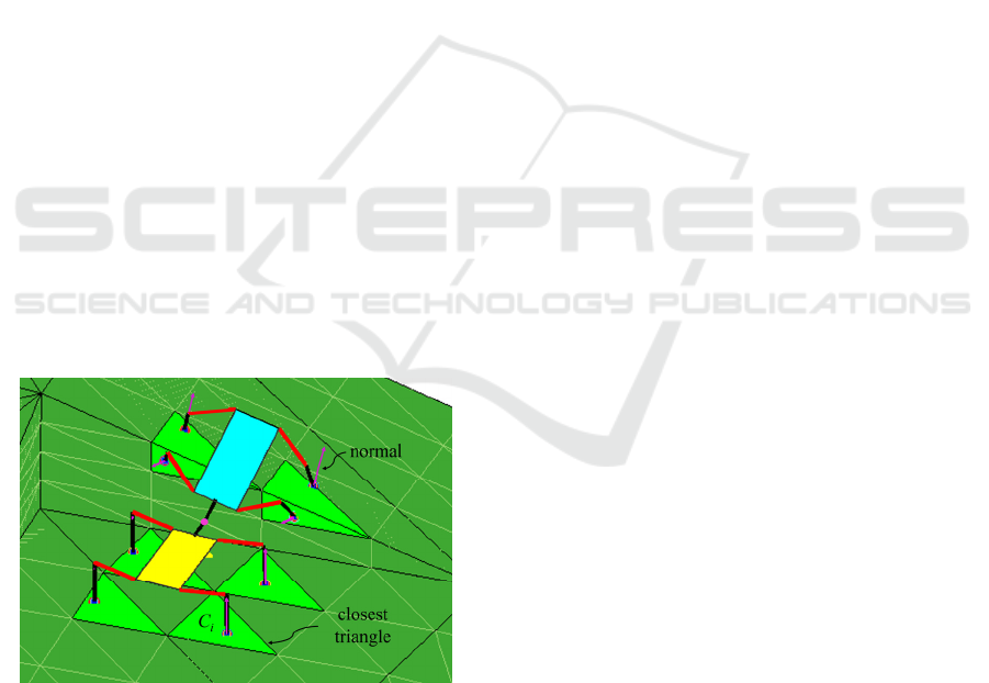
One of the objectives of the article is to identify

the location of the robot's footholds on the subdivided

terrain. To achieve this, the triangle of the terrain

closest to each foot of the robot is found and a

projection of the foot onto this triangle is made. This

process is repeated for each of the robot's legs.

Figure 2: a) Original terrain. b) Subdivided terrain.

Initially, a brute force search was used to find the

closest triangle by checking all triangles in the

environment. However, this approach proved

computationally expensive. To improve the search

process, we decide to examine only triangles that are

within a short distance of the robot's shoulder. To do

this, a k-d tree is created using the centroids of the

subdivided triangles that make up the terrain.

Through this k-d tree, the centroids that lie within a

sphere centred at the shoulder of the leg, with a radius

of r*1.5, are determined. In this case, r has a value of

0.2, corresponding to the total length of the robot leg

when fully extended.

Once the triangle closest to the foot of each leg

has been identified, the projection of each foot on the

closest triangle is calculated. This ensures that the

robot, in each position, has all its legs correctly

supported on the ground, which makes it possible to

analyse its stability, as described in the next section.

4 STABILITY ANALYSIS

Stability plays a crucial role in the robot's path

planning, since if it moves along an unstable path, it

could face tipping or slipping situations,

compromising both its safety and accuracy in task

execution.

In order to guarantee the stability of the robot, it

is essential to carry out an analysis of the support

points. The Zero Moment Point (ZMP) is the point at

which the reaction forces produced at the robot's

contacts with the ground do not generate any moment

ICINCO 2023 - 20th International Conference on Informatics in Control, Automation and Robotics

650

in the horizontal direction. In planar horizontal

grounds with sufficient friction, the ZMP must be

within the convex hull of the robot's contact points

with the ground for the robot to be in a stable position.

However, this analysis becomes more complex for

robots with multiple non-coplanar contacts, or when

friction is not sufficiently high to neglect slippage. In

this context, Hirukawa et al. (2006) proposed a more

general stability criterion based on the Contact

Wrench Cone (CWC), which addresses this issue by

considering the friction constraints between the

contact points and the ground.

In this method, the stability of a contact point C

is evaluated by the contact force f

, which is the vector

sum of the normal reaction along the normal n

at the

contact point, and the friction force tangent to the

ground, f

friction

. For a contact point to be considered

stable, the contact force is required to be within the

friction cone, defined as:

‖𝐧



 𝐟



𝐧



‖



 𝜇





𝐟



𝐧





(1)

where 𝜇



is the coefficient of friction.

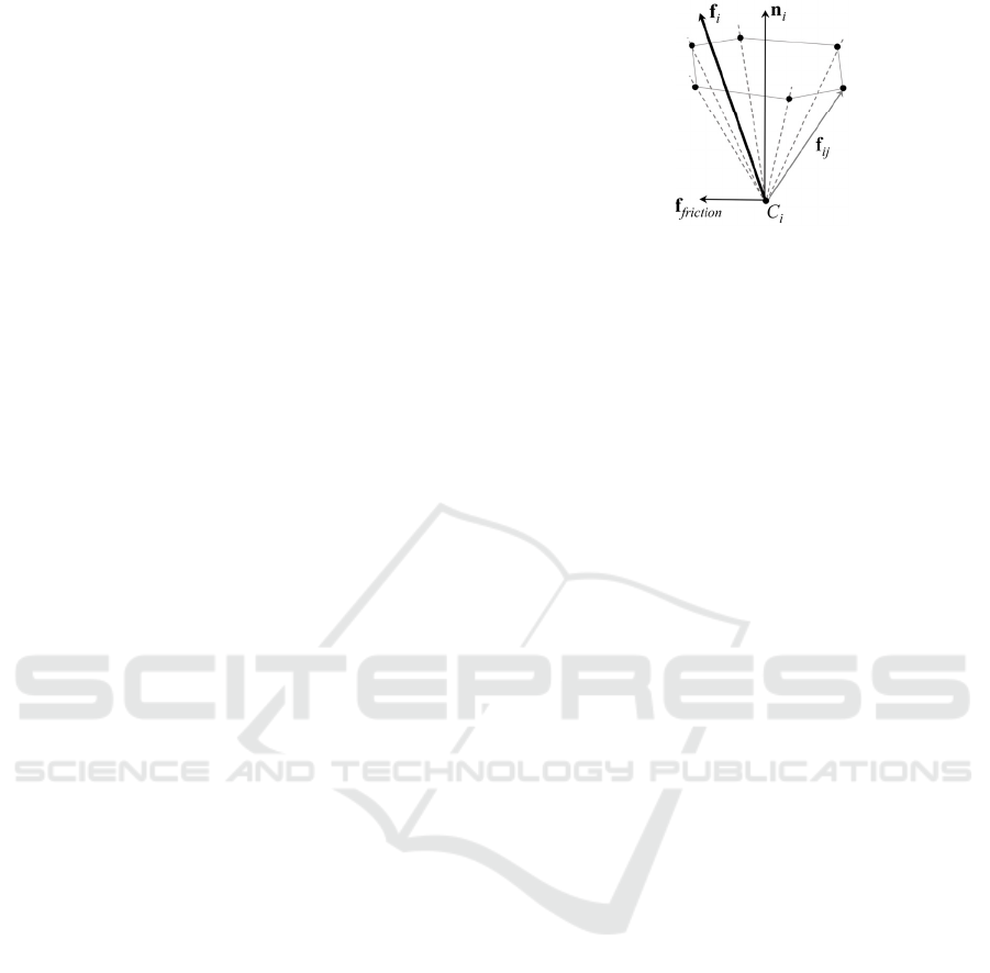
In numerous articles, such as (Caron et al. 2017),

a linear approximation of the friction cone is used due

to its better computational efficiency in terms of

computational speed and processing. This

approximation consists in approximating the cone by

an inner pyramid whose lateral edges are denoted by

, as shown in Figure 3. To ensure the stability of the

robot, condition (2) must be fulfilled, which involves

the f

vectors and their moments, considering the

position of C

in relation to the global coordinate

system, defined as p



𝐟

𝛕



𝜆





𝐟



𝐩





𝐟



 𝜆



0

(2)

where the subscript i iterates over the contact points

(i = 1 … 8 for the legged robot described in Section

2) and j iterates over the edges used in the

approximation of the friction cones by pyramids.

Equation (2) establishes that the resultant of the

external forces 𝐟 and moments 𝛕



(due to gravity,

inertia, etc.) that could cause the robot to tip over or

slip, must be a linear combination of the vectors f

and their moments, multiplied by non-negative

coefficients 𝜆



. This ensures the stability of the robot

by guaranteeing that the f

reactions are within the

friction pyramid. In this article, 10 f

vectors have

been used to approximate the friction cone at each

contact point, although for simplicity only 6 edges are

represented in Figure 3.

Figure 3: Stable Contact C

Typically, the stability test consists in building the

6-dimensional CWC cone represented by the right-

hand side of (2), and checking if the left-hand side of

(2), i.e., the 6-dimensional vector [𝐟 ; 𝛕



], belongs to

this CWC, in which case the robot is stable. However,

building the CWC is a costly operation, and in this

paper we will use a simpler method to check if (2)

admits a solution consisting of non-negative 𝜆



for a

given wrench [𝐟 ; 𝛕



], as explained next.

The stability test employed in this paper begins by

transforming the inequality constraints of (2) into

equivalent equalities, by defining a new auxiliary

variable 𝑡



for each 𝜆



, and then replacing each

inequality 𝜆



0 by its equivalent quadratic

equation:

𝜆



𝑡





(3)

After this, (2) becomes a quadratic system of six

equations with many more than six unknowns 𝜆



and

𝑡



(e.g., if each friction cone is approximated by a 10-

sided pyramid, and having eight contact points, we

have 80  2 unknowns 𝜆



and 𝑡



). This

underdetermined system is solved by the iterative

Newton-Raphson method, using the pseudoinverse of

the Jacobian matrix that gives the least norm solution.

If we make several attempts (e.g., 10) to obtain a

converging solution using the Newton-Raphson

method as explained above, where each attempt starts

from a different random value of 𝜆



and 𝑡



, and all

attempts fail to converge after a reasonable number of

iterations, then we conclude that the robot is unstable,

as it is impossible to find non-negative 𝜆



that satisfy

(2) for the given left-hand side [𝐟 ; 𝛕



]. Otherwise, if

at least one attempt converges to a solution, then we

conclude that the robot is stable.

By running several examples where stability was

tested using the described Newton-Raphson method

or the typical method that requires building the 6-

dimensional CWC, we checked that both methods

always gave the same verdict of stability, but the

Newton-Raphson method performed roughly 10

times faster, and it was easier to implement. This

Simultaneous Planning of the Path and Supports of a Walking Robot

651

higher speed is advantageous if the stability test must

be repeatedly performed many times, as it will be

required in the path-planning algorithm described in

the next Section. Therefore, in the following, we will

test stability using the Newton-Raphson method

described above.

5 PLANNING THE PATH AND

CONTACT POINTS

The aim of this paper is to perform simultaneous

planning of the path and locations of footholds of the

multi-legged robot introduced in Section 2. To

achieve this, we implement the A-star search

algorithm (A*), which searches for the path with the

lowest cost from an initial position to a final position.

We use the A* algorithm to find a sequence of

waypoints of the terrain at which the robot can be

positioned and oriented stably without suffering

tipping over or slipping, with all its eight feet

supported on the terrain. We do not solve, however,

the sequence of movements that the robot needs to

execute to move from one waypoint to the next one,

i.e., lifting and swinging each leg to move the robot

while other legs rest on the terrain. This latter

problem is left for future work.

In our approach, we start from a terrain

subdivided into triangles, whose known centroids

form a grid of points that serves as the search space

for the algorithm. Using these points, a k-d tree is

constructed and used at the beginning of the

algorithm to find the initial and final nodes closest to

the desired initial and final positions provided by the

user or high-level path planner. In addition, while the

algorithm executes the steps described later, the same

k-d tree is also used to find the n nearest neighbour

nodes to the current node, where in this example, n is

equal to 10. The use of k-d trees allows us to make

these searches more efficiently compared to an

exhaustive brute-force search.

In this paper, in order to obtain the optimal route,

the A* algorithm is used to carry out an exploration

along all the centroids (nodes) of the triangles

representing the terrain. A variant of the conventional

A* algorithm is used, where the distances or costs

associated with each node are modified, taking into

consideration both the stability of the robot and the

similarity between the configurations or postures

adopted by the robot between neighbour nodes. The

algorithm implemented in this article can be

summarised in the following steps:

1) The algorithm explores all the nodes that are

part of the terrain map, starting with the initial

node and prioritising the search among those

nodes with the lowest cost

𝑓 (the definition of

cost

𝑓 will be provided later).

2) After that, the 10 nearest neighbour nodes to

the current node are determined (initially, the

current node is the initial node).

3) The costs

𝑓 and 𝑔 are obtained for each of the

neighbouring nodes that have not been

previously evaluated or explored.

𝑔 𝑛𝑒𝑖𝑔ℎ𝑏𝑜𝑢𝑟𝑔𝑐𝑢𝑟𝑟𝑒𝑛𝑡  𝑑 𝑞 𝑒

𝑓

𝑛𝑒𝑖𝑔ℎ𝑏𝑜𝑢𝑟𝑔𝑛𝑒𝑖𝑔ℎ𝑏𝑜𝑢𝑟  ℎ

(4)

where:

- 𝑔𝑥 represents the real cost of reaching node

“𝑥” from the initial node.

- 𝑓



𝑛𝑒𝑖𝑔ℎ𝑏𝑜𝑢𝑟



is an estimate of the total cost of

going to the destination node from the initial node,

passing through the

𝑛𝑒𝑖𝑔ℎ𝑏𝑜𝑢𝑟 node. This cost is

calculated using a distance heuristic ℎ that must not

overestimate the actual distance. In this case, for

simplicity, the straight-line distance between the

𝑛𝑒𝑖𝑔ℎ𝑏𝑜𝑢𝑟 and the destination is used as the heuristic

ℎ.

- 𝑑 is the actual distance between the

𝑐𝑢𝑟𝑟𝑒𝑛𝑡

node and the

𝑛𝑒𝑖𝑔ℎ𝑏𝑜𝑢𝑟.

- 𝑞 represents the difference between the

configurations adopted by the robot when resting at

the

𝑐𝑢𝑟𝑟𝑒𝑛𝑡 node and at the 𝑛𝑒𝑖𝑔ℎ𝑏𝑜𝑢𝑟 node. The

difference in positions and orientations of the robot's

modules, as well as the joint angles rotated by its legs,

between the posture at the

𝑐𝑢𝑟𝑟𝑒𝑛𝑡 node and at the

𝑛𝑒𝑖𝑔ℎ𝑏𝑜𝑢𝑟 node is considered. The objective is to

minimise 𝑞 to try to achieve continuity in the postures

adopted by the robot along the various nodes it travels

during the path.

- 𝑒 is a penalty for lack of stability. By applying

the method described in Section 4, the stability of the

robot when placed on the

𝑛𝑒𝑖𝑔ℎ𝑏𝑜𝑢𝑟 node is

evaluated. In situations where instability is identified,

a significantly high value is assigned to

𝑒 as a penalty,

so that the A* algorithm will discard that node as part

of the potential path to the destination node. In

contrast, if the robot is stable,

𝑒 is set to 0.

It is important to consider that 𝑞 and 𝑒 are

dependent on the orientation adopted by the robot

when it is positioned over the

𝑛𝑒𝑖𝑔ℎ𝑏𝑜𝑢𝑟 node. To

tackle this, four orientations separated by 45 degrees

are explored, as it will be explained later. The

orientation that yields the lowest value for the sum of

𝑞 and 𝑒 is selected.

The next subsection details the process of

"building" the robot's posture as it is placed over each

ICINCO 2023 - 20th International Conference on Informatics in Control, Automation and Robotics

652

𝑛𝑒𝑖𝑔ℎ𝑏𝑜𝑢𝑟 node. This is done in order to evaluate all

the previously mentioned costs.

5.1 Building the Posture of the Robot

at Each Node

To calculate the different costs involved in (4), the

robot must be placed at a given position with all eight

feet resting on the ground. This requires defining the

footholds for all feet, the position and orientation of

the central body of each of the two modules that

integrate the robot, and the joint angles of every leg.

This subsection will describe the calculations that

allow us to define a reasonable and feasible posture

of the robot when placed over each node visited by

the A* algorithm. This feasible posture will be

obtained by first building a tentative posture, and later

refining it using Newton-Raphson iterations, to

guarantee that all feet of the robot rest on the ground.

First, the spherical or ball joint connecting the two

robot modules, called C, is placed at a distance a from

the node or centroid of the triangle being evaluated,

along the direction normal n to the triangle. Then, a

principal axis called ep is defined, which is taken as

any vector perpendicular to the normal n. This vector

ep represents the main axis of the robot, i.e., the axis

along which both bodies depicted in Figure 1 would

be aligned if the robot adopted a posture so symmetric

and “straight” as that shown in Figure 1. Evidently,

since the terrain over which the robot moves is not

flat, the final posture adopted by the robot at each

node (this final posture will be constructed in the

following paragraphs of this section) will not be so

symmetric and straight as in Figure 1, but it will still

be somewhat oriented in the direction of ep.

After aligning the bodies with the principal axis

ep, the coordinate frames of each body, which define

the orientation of each body, are calculated as shown

in Figure 4. To this end, the bodies are arranged

perpendicular to the normal n

of the triangle located

directly below the centre of each body

i. The normal

of the body corresponds to the z-axis, while the x-axis

is defined as the normalized projection of the

principal axis ep on the plane of the body. Finally, the

y-axis is obtained by the cross product of the z-axis

and the x-axis.

In addition, the centres of the bodies are

determined as the intersection between each of the x-

axes of the bodies (regarded as infinite lines passing

through the spherical joint C) and a sphere of radius

𝑅, centred at C, as illustrated in Figure 5.

The intersection points between the sphere and the

x-axes gives:

𝑥



𝑥



𝑅𝑥

,

𝑦



𝑦



𝑅𝑥

,

𝑧



𝑧



𝑅𝑥

,

(5)

where 𝑅𝑙 𝐿



/2 is the sum of the length 𝑙 of the

little segment that joins each body to the spherical

joint C, and L

is the length of each body along its x-

axis. On the other hand, x

, y

and z

correspond to

position of joint C, while the coordinates 𝑥



, 𝑦



, 𝑧



represent the centre of body i. 𝑥

,

, 𝑥

,

, and 𝑥

,

are the components of the unit vector of the x-axis of

each body i.

Figure 4: Central bodies of the robot without legs in the ep

direction.

Figure 5: Intersection of the sphere centred at C with the x-

axis of each body.

After defining the position and orientation of each

body, the four legs are added to each body. Initially,

these legs are added forming exactly a right angle

with respect to the body, similar to the legs of the

yellow body shown in Figure 6. Note that, if the

terrain under the bodies of the robot is not flat for the

node that is being evaluated, in general, some of the

feet may not be in contact with the terrain after

placing the legs at right angles as indicated here.

Indeed, if the terrain below the body is concave, some

legs may penetrate under the terrain, and if the terrain

is convex, some feet may be in the air above the

terrain, not touching it. However, this is not a problem

because the final posture of the robot will be corrected

using the Newton-Raphson method as explained later,

Simultaneous Planning of the Path and Supports of a Walking Robot

653

so that it correctly rests on the terrain, with all feet in

contact with the ground.

The penultimate operation to build the tentative

posture of the robot when placed over each node

consists in finding the points of contact where each

foot should be placed (as said in the previous

paragraph, some feet may be under the terrain if it is

concave, or over it if it is convex). This is done by

finding the projection of each foot on the closest

triangle of the terrain, as explained at the end of

Section 3. These projections are the footholds where

each foot should be placed.

Finally, the last operation to complete the

calculation of the posture of the robot when placed

over each node of the terrain, consists in defining a

set of loop-closure equations that represent the

following constraints: each foot of the robot should

be placed at the corresponding closest foothold, and

both bodies should be joined by the spherical joint C.

These constraints define a system of nonlinear

equations whose unknows are the position and

orientation coordinates of each body, as well as the

joint angles (q

, q

) of each leg (recall these joint

angles in Figure 1). This nonlinear system is solved

using the Newton-Raphson method, starting the

iterations from the tentative posture built by

following all the operations described in this

subsection 5.1. The result of these iterations is a

realistic and feasible posture of the robot with both

bodies joined at C and all feet resting on the ground,

as illustrated in Figure 6. This feasible posture will be

similar to the tentative posture which is used as the

seed of the Newton-Raphson iterations.

Figure 6: The robot with all its legs resting on the ground.

Once the robot adopts a feasible posture on the

ground, its stability is tested using the method

described in Section 4, obtaining the sub-cost 𝑒 used

in (4). The difference between this posture at the

current node and that at its neighbour is also

calculated, to obtain the value of the sub-cost 𝑞 used

also in (4). All calculations described in this

subsection 5.1 are repeated three more times, but each

time rotating the main axis ep about n by 45º with

respect to the previous time, so that different postures

of the robot are tested to roughly cover all possible

orientations about axis n, finally retaining the posture

that gives a smaller value of 𝑒𝑞. This is added to

the sub-costs 𝑑 and ℎ of (4), to complete the

calculation of the cost at each node, making it

possible for the A* algorithm to determine the

shortest route to move from a starting point to an end

point.

After executing the A* algorithm, it returns the

centroids of the subdivided triangles of the terrain that

form part of the optimal path, the information of the

posture of the robot at each node of the optimal path

(orientations and positions of the central bodies and

joint angles of the legs), and the support points for all

legs, at each node. This will be illustrated with some

examples in the next section.

6 RESULTS

The evaluation of the effectiveness of the algorithm

A* for calculating the path and the determination of

the robot positions and contact points has been carried

out in this Section 6. For this purpose, two examples

have been studied, which are significant and

representative for the method because they require the

robot to climb or descend an irregular terrain with

several slopes. For each example, an initial and a final

position have been defined, and the resulting paths

have been compared, considering or ignoring the

influence of the stability of the robot in each position

until the target position is reached. In the study, a

friction coefficient of 0.4 has been considered.

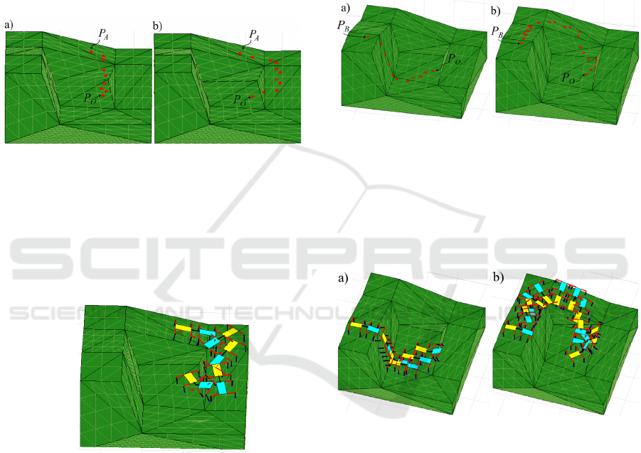
In the first study, the robot must ascend the first

ramp and reach an intermediate position on the

second ramp (P

[0, 0.75, -0.2]), starting from an

initial position in the lowest part of the terrain (P

[0,

0, -0.5]). To evaluate the optimal path from P

to P

without taking stability into account, Figure 7a, the

A* algorithm takes 135 seconds to find the path (this

algorithm was implemented in Matlab 2015a on

Windows, and it was run on an Intel(R) Core(TM) i7-

8750H CPU @ 2.20 GHz processor with 16 GB

RAM). The red dots in Figure 7 represent the

centroids of the triangles forming part of the optimal

path where the projection of the centre of the robot's

bodies, C, would be placed and the robot's position

would be constructed as explained in section 5.1. The

path obtained (Figure 7a) shows how the robot goes

straight up to P

on the steep part of the second ramp,

ICINCO 2023 - 20th International Conference on Informatics in Control, Automation and Robotics

654

where we should expect that the robot would lose

stability and tip over or slip, as the next simulation

confirms.

On the other hand, when stability is taken into

account for optimal path finding, Figure 7b, the robot

goes up the ramps that have an inclination that does

not compromise its stability, even though this implies

a longer path. In that case, the algorithm requires a

response time of 544 seconds to find the optimal path.

However, this path ensures that the robot is stable

throughout the entire route, avoiding possible tipping

or slipping problems.

Figure 7: a) Optimal path of the robot from P

to P

without

stability (red dots). b) With stability.

Furthermore, the A* algorithm simultaneously

provides the robot's positions and the contact points

at each node of the obtained path. Figure 8 shows

some of the robot positions along the path shown in

Figure 7b, considering the stability and orientation of

the robot.

Figure 8: Positions and contacts of the robot in the path to

In the second example studied, the optimal path is

calculated for the robot to descend from the highest

point of the terrain

[-1, -0.4, 0.2] to the point P

Figure 9. Note that this example requires the robot to

traverse most of the terrain and, therefore, it includes

other example paths in which the robot may need to

travel between intermediate points of the terrain.

On the one hand, similar to the previous example,

the robot path is calculated using the A* algorithm

without taking stability into account, Figure 9a. In

this case, the algorithm takes 247 seconds to

determine the path with the lowest cost, which is the

one that goes straight to P

down the ramp with a

steep slope where the robot would evidently not be

stable and would tip over.

On the other hand, when considering the stability

of the robot in the path calculation (Figure 9b), the

response time of the algorithm increases significantly,

reaching approximately 1 hour and 9 minutes. This is

because the robot must avoid going straight down the

steep ramp to maintain its stability. Instead, it needs

to travel a longer path, involving more nodes, to reach

the end point safely.

Figure 9: a) Optimal path of the robot from P

to P

without

stability (red dots). b) With stability.

Figure 10 shows some of the robot positions

(postures and contact points) going through the

optimal robot path obtained by algorithm A* to reach

from the position P

ignoring robot stability,

Figure 10a, and considering stability, Figure 10b.

Figure 10: a) Positions and contacts of the robot in the path

to P

without stability. b) With stability.

The algorithm was run again to plan a path from

to P

, i.e. to climb the terrain instead of descend

it, and it took 1hour and 42 minutes, which is about

30 minutes more than the time taken to compute the

descending path. More simulations were run between

initial and final points near P

and P

, and in all of

them we observed that the time to find an ascending

path was slightly higher than to find a descending

one. This can be explained by the fact that, when

starting up, many of the nodes of the terrain belong to

steep slopes at which the robot is unstable, so the

search is more directed than when starting down,

where the nodes yield stable postures and there are

more options to explore.

Simultaneous Planning of the Path and Supports of a Walking Robot

655

7 CONCLUSIONS

This paper describes a method for path planning of

multi-legged robots in irregular environments. To

tackle this challenge, a method has been proposed that

starts with the creation of a triangular mesh to define

the contact points of the legs and establish a mesh of

nodes for path planning. After this, the A* algorithm

has been used to find the optimal path from an initial

position to the target position, ensuring that the robot

maintains stability along the path and adopts realistic

and coherent configurations.

This method has also made it possible to identify,

at each point in the path, the robot's contact points and

postures, providing a representation of its positions in

the environment.

However, considering that the robot will need to

plan the next path while it executes the current one, it

will be crucial to improve the search times of the

current algorithm. In this context, a promising

strategy to increase efficiency is to explore the use of

Rapidly Exploring Random Trees (RRT) instead of

the A* algorithm. Although the A* algorithm is

capable of finding the absolute optimal path, its high

computational cost limits it in applications requiring

real-time computations. On the other hand, the RRT

algorithm offers faster search times, although the

solutions found may be sub-optimal compared to the

exhaustive approach of the A* algorithm.

As another future line of research, it will be

necessary to address the planning of the movements

between successive postures, i.e.: for every two

neighbouring postures of the optimal path obtained by

the algorithm, it will be necessary to determine a

sequence of movements to transform one posture into

another (sequence of raising and swinging legs, etc.),

while keeping stability.

ACKNOWLEDGEMENTS

This work is part of the INVESTIGO 2022

Programme (file number: INVEST/2022/432) funded

by the Valencian Conselleria d’Innovació,

Universitats, Investigació i Societat Digital, and by

the European Union (Next Generation EU); and of the

CIGE/2021/177 project, funded by the Valencian

Conselleria d’Innovació, Universitats, Ciència i

Societat Digital.

REFERENCES

Aceituno-Cabezas, B., Dai, H., Cappelletto, J., Grieco, J.

C., Fernández-López, G. (2017). A mixed-integer

convex optimization framework for robust multilegged

robot locomotion planning over challenging terrain. En:

2017 IEEE/RSJ International Conference on Intelligent

Robots and Systems, pp. 4467–4472.

Aceituno-Cabezas, B., Mastalli, C., Dai, H., Focchi, M.,

Radulescu, A., Caldwell, D. G., Cappelletto, J., Grieco,

J. C., Fernández-López, G., Semini, C. (2018).

Simultaneous contact, gait, and motion planning for

robust multilegged locomotion via mixed-integer

convex optimization. IEEE Robotics and Automation

Letters 3(3), 2531–2538.

Caron, S., Kheddar, A. (2016). Multi-contact walking

pattern generation based on model preview control of

3D CoM accelerations. In 2016 IEEE-RAS 16th

International Conference on Humanoid Robots, pp.

550–557.

Caron, S., Pham, Q. C., Nakamura, Y. (2017). ZMP support

areas for multicontact mobility under frictional

constraints. IEEE Transactions on Robotics 33(1),67–

80.

Dai, H., Tedrake, R. (2016). Planning robust walking

motion on uneven terrain via convex optimization. En:

2016 IEEE-RAS 16th International Conference on

Humanoid Robots, pp. 579–586.

Ellenberg, R. W., Oh, P. Y. (2014). Contact wrench space

stability estimation for humanoid robots. In 2014 IEEE

International Conference on Technologies for Practical

Robot Applications, pp. 1–6.

Hirukawa, H., Hattori, S., Harada, K., Kajita, S., Kaneko,

K., Kanehiro, F., Fujiwara, K., Morisawa, M. (2006). A

universal stability criterion of the foot contact of legged

robots-Adios ZMP. En: 2006 IEEE International

Conference on Robotics and Automation, pp. 1976–

1983.

Jenelten, F., Grandia, R., Farshidian, F., Hutter, M. (2022).

TAMOLS: Terrain-aware motion optimization for

legged systems. IEEE Transactions on Robotics 38(6),

3395–3413.

Li, S., Chen, H., Zhang, W., & Wensing, P. M., (2022). A

geometric sufficient condition for contact wrench

feasibility. IEEE Robotics and Automation Letters 7(4),

12411–12418.

Navaneeth, M. G., Sudheer, A. P., Joy, M. L. (2022).

Contact wrench cone-based stable gait generation and

contact slip estimation of a 12-DOF biped robot.

Arabian Journal for Science and Engineering 47,

15947–15971.

Orsolino, R., Focchi, M., Mastalli, C., Dai, H., Caldwell, D.

G., Semini, C. (2018). Application of wrench-based

feasibility analysis to the online trajectory optimization

of legged robots. IEEE Robotics and Automation

Letters 3(4), 3363–3370.

Vukobratović, M., Borovac, B. (2004). Zero-moment

point—thirty five years of its life. International Journal

of Humanoid Robotics 1(1), 157–173.

ICINCO 2023 - 20th International Conference on Informatics in Control, Automation and Robotics

656