Exploring Segnet Architectures for iGPU Embedded Devices
Jean-Baptiste Chaudron
a
and Alfonso Mascarenas-Gonzalez
b
ISAE-SUPAERO, Universit
´
e de Toulouse, France
Keywords:
CNN, iGPU, Segnet, Embedded Systems.
Abstract:
Image segmentation is an important topic in computer vision which encompasses a variety of techniques to
divide image into multiple areas or sub-regions in order to extract meaningful information. Artificial Neural
Networks (ANNs), biologically inspired algorithms, are nowadays widely used to perform such tasks and
popular models are usually based on encoder-decoder architectures. Segnet was one of the first proposed
model of this kind in the literature and, despite its efficiency, it has several drawbacks for embedded systems
especially due to the huge amount of arithmetic operations and memory used in the original version. However,
its simple sequential based architecture offers interesting properties for optimization and real-time analysis. In
this paper, we deeply investigate how to tune and adapt original Segnet architecture to allow efficient run-time
execution on embedded targets equipped with an iGPU. We propose our own implementation design which
is experimented and validated on iGPU embedded devices for two state of the art datasets from Unmanned
Aerial Vehicle (UAV) applications.
1 INTRODUCTION
Image segmentation consists of variety of techniques
deployed in many computer vision applications such
as autonomous car driving or Unmanned Aerial Ve-
hicle (UAV) technologies (Osco et al., 2021). The
problem is very complex due to the handling of fine
granularity information within images, consequently,
image segmentation has been a research area for years
and several techniques as well as algorithms have
been proposed (Zaitoun and Aqel, 2015) such as:
• Region based methods using threshold algo-
rithms Otsu threshold (Otsu, 1979), minimal er-
ror threshold (Deravi and Pal, 1983) or k-means
algorithms (Dhanachandra et al., 2015);
• Edge detection techniques like well known Canny
and Sobel filters (Canny, 1986; Kanopoulos et al.,
1988) or by exploiting partial differential equa-
tions to capture edges boundaries (Sli
ˇ
z and
Mikulka, 2016).
Over the past few years, the use of Artificial
Neural Network (ANN), and especially Convolutions
Neural Network (CNN), models have become more
and more popular for image segmentation showing
significant performance improvements compared to
a
https://orcid.org/0000-0002-2142-1336
b
https://orcid.org/0009-0006-7355-1809
more traditional approaches (Mahony et al., 2019).
However, the more accurate an ANN model is, the
larger it gets and uses more processing power which
can make a very efficient ANN model impossible
to execute without dedicated hardware accelerators.
Nowadays, Graphics Processing Units (GPUs), ini-
tially designed for graphic rendering, are the most
widely used ANN hardware accelerators outperform-
ing traditional processors for such tasks (Strigl et al.,
2010). The main provider of GPU solutions is
NVIDIA which has known a huge expanse in the
use of its GPU technology thanks to the development
of CUDA, a low level language similar to C++, used
for directly programming fine grain functionalities
on their GPUs. NVIDIA also offers several scaled-
down GPU versions which are combined with an
ARM CPU for edge and embedded devices systems
(i.e. integrated GPUs or iGPUs). Moreover, many
deep learning frameworks are available and compli-
ant with CUDA and NVIDIA devices (Hatcher and Yu,
2018). These frameworks provide a set of easy-to-use
libraries to speed up the development and the integra-
tion of ANN solutions on all platforms. However, the
use of iGPU architectures in safety critical embedded
systems raise several challenges such as the real-time
determinism behavior (Perez-Cerrolaza et al., 2022).
To ensure real-time behavior of a CNN algorithm run-
ning on an iGPU, it is mandatory to have a full under-
Chaudron, J. and Mascarenas-Gonzalez, A.
Exploring Segnet Architectures for iGPU Embedded Devices.
DOI: 10.5220/0012185100003595
In Proceedings of the 15th International Joint Conference on Computational Intelligence (IJCCI 2023), pages 419-430
ISBN: 978-989-758-674-3; ISSN: 2184-3236
Copyright © 2023 by SCITEPRESS – Science and Technology Publications, Lda. Under CC license (CC BY-NC-ND 4.0)
419

standing of the model and to have a full control on its
implementation using low level primitives.
The work presented in this paper offers a deep
analysis of the encoder-decoder Segnet architecture
for image segmentation. We choose this CNN model,
because of its simple sequential architecture based on
well known arithmetic operations that can be opti-
mized. We discuss its original structure and investi-
gate how to customize it to build more efficient mod-
els. In particular, we describe our implementation de-
tails and present some experimental results based on
two semantic segmentation datasets from UAV appli-
cations. In addition, an accurate bibliography is pre-
sented throughout this document to support our ap-
proach. This paper is organized as follow:
• Section 2 explains the background with the emer-
gence of CNNs architectures for semantic seg-
mentation and the challenge of their integration
on embedded systems.
• Section 3 explores the Segnet original architec-
ture, describes our proposed customizations, de-
tails the training environment and presents the
corresponding results.
• Section 4 investigates iGPU design considera-
tions, shows our experimental results on hard-
ware devices and, finally, Section 5 concludes and
offers some possible perspectives to pursue our
work.
2 STATE OF THE ART
2.1 Emergence of CNNs
ANNs can be seen as computational data processing
systems inspired by the biological way nervous sys-
tem operates. In 1957, the first approach to implement
a neural network, called the perceptron, has been pre-
sented (Rosenblatt, 1957). Then, this first approach
has been improved with extensions to multiple lay-
ers (Irie and Miyake, 1988) called Multi-Layers Per-
ceptron (MLP) or Fully Connected Network (FCN).
For pattern recognition applications, this basic linear
architecture was not capable to capture geometric 2-
Dimensional (2D) relationships within an image. In
1980, the concept of the neocognitron (Fukushima,
1980) introduced an innovative structure with a con-
cept that will become the core of CNNs by process-
ing an image by regions and performing the same op-
erations on all the regions of the image. Then, fol-
lowing some principles from the neocognitron and,
also, integrating learning capabilities developed for
MLPs (Rumelhart and McClelland, 1987; Yam and
Chow, 1993), the first application of CNNs was im-
plemented in 1998 (Lecun et al., 1998) for an hand-
written digit recognition task (the MNIST dataset
1
).
The difference between MLP and CNN architectures
for the MNIST data-set is illustrated in Figure 1 where
we can observe the 2D relationships handling of a
CNN model versus the linear approach proposed by
a MLP model.
Figure 1: Illustration of MLP and CNN for MNIST.
2.2 From Classification to Segmentation
From this first CNN effort applied to the MNIST
dataset, a sharp increase of the development and de-
ployment of CNN based techniques for image clas-
sification has occurred. The availability of many
other datasets like CIFAR
2
and challenges such as
ILSVRC
3
(Russakovsky et al., 2015) led to a sig-
nificant improvement of CNN based computer vision
models and architectures, for instance well known
AlexNet (Krizhevsky et al., 2012), VGG (Liu and
Deng, 2015) or Resnet (He et al., 2016). All these ar-
chitectures are very accurate for image classification
but can’t be applied directly to image segmentation.
Indeed, as illustrated in Figure 2, semantic segmenta-
tion extends classification because instead of deter-
mining if an image belongs to a certain class, the
model must detect to which class each pixel of the
input image belongs to (i.e. all pixels in the image
are labeled to a corresponding class). Note that, for
both classification and segmentation, the original im-
age often needs to be down-sampled in order to limit
the memory usage and the number of arithmetic oper-
ations (Hirahara et al., 2021).
Image segmentation is a more complex task that
requires updated CNN models and methods. Several
solutions have been proposed in the literature over the
1
http://yann.lecun.com/exdb/mnist/
2
https://www.cs.toronto.edu/
∼
kriz/cifar.html
3
https://www.image-net.org/challenges/LSVRC/
NCTA 2023 - 15th International Conference on Neural Computation Theory and Applications
420

Figure 2: Comparison of Classification and Segmentation.
years such as Fully Convolutional Networks (FCNs)
(Long et al., 2015); Pyramid Network Based Models
like Feature Pyramid Networks (FPNs) or Pyramid
Scene Parsing Networks (PSPNs) (Lin et al., 2017;
Zhao et al., 2017); encoder-decoder models with
simple convolutions usage such as Segnet (Badri-
narayanan et al., 2017), analyzed in this paper, or with
more complex structures including dilated and trans-
posed convolutions like Enet (Paszke et al., 2016)
or Erfnet (Romera et al., 2018). Many others ANN
based techniques as well as methods are also avail-
able (Minaee et al., 2022).
2.3 Embedding Semantic Segmentation
Deep learning frameworks bring easy-to-use libraries
for the design and deployment of ANN solutions on
many platforms (Hatcher and Yu, 2018). In particu-
lar, some of these frameworks provide optimized ver-
sions for embedded devices such as cuDNN (Chetlur
et al., 2014) or TensorRT (Jeong et al., 2022) and their
performances for inference have been tested in sev-
eral works (Lee et al., 2022; Zelek and Jeon, 2022).
The use of these libraries is the current paradigm to
deploy ANN based solutions on embedded systems.
However, deployment of semantic segmentation mod-
els in areas such as autonomous vehicles and UAV
applications may not only require performance but it
is also mandatory to ensure real-time properties, i.e.
the model needs to have a deterministic behavior for
its execution. The challenges of addressing real-time
properties is complex and amplified by the need to op-
erate on resource constrained hardware components.
Therefore, the need of predictability in critical sys-
tems requires a full understanding of the execution
platform architecture we are working with (NVIDIA,
2022; NVIDIA, 2023), the behavior of the function
(especially the handling of the memory), the schedul-
ing of the task/kernels (Amert et al., 2017) and the
interface between the CPU and the iGPU (synchro-
nization, data transfer, ...) (Yang et al., 2018). For
these reasons, we decided to implement our own low
level CUDA based solution for the Segnet architecture
in order to have a full control on all these mentioned
aspects going from design to implementation.
3 EXPLORING SEGNET
ARCHITECTURES
3.1 Original Architecture Overview
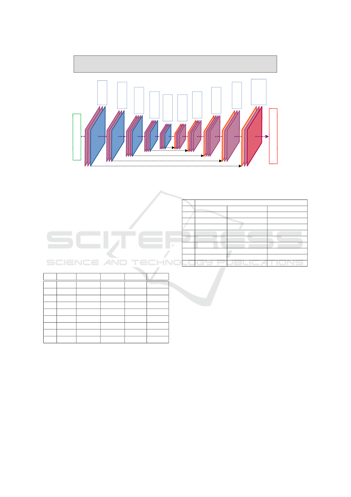
The original Segnet architecture (Badrinarayanan
et al., 2017) is based on a fully sequential and sym-
metric encoder-decoder architecture as depicted in
Figure 3. The encoder and the decoder consists of
5 levels of convolution and batch normalization lay-
ers (Ioffe and Szegedy, 2015) with Relu activation
(noted CBNR in Figure 3). Each CBNR layer is
followed by a max pool layer for the encoder part
or preceded by a max unpool layer for the decoder
part. The max pool layers are sharing the indexes with
their symmetric max unpool layers for more accuracy
while decoding. Each convolution layer is using sim-
ple convolution based on 3×3 filters very convenient
for optimization (see Section 4.2). Note that the very
last layer contains an additional softmax activation to
allow having a probability distribution over the differ-
ent classes for each pixel, thus the number of output
classes depends on the targeted segmentation applica-
tion (see Section 3.3). The Segnet model is very simi-
lar to Unet (Ronneberger et al., 2015) which uses con-
catenation between feature maps from encoder and
decoder levels and where indexes are not shared be-
tween encoder max pool and decoder max unpool lay-
ers. Segnet can also be compared to DeconvNet (Noh
et al., 2015) with an identical encoder part but using
deconvolutions for the decoder.
3.2 Towards New Architectures
The original Segnet architecture is greedy in terms
of computing resources (memory, processing) and
is usually limited for embedded system applica-
tions. However, its simple sequential architecture
and the use of basic 3×3 convolutions can be highly
optimized (see Section 4.2) using Winograd meth-
ods (Lavin and Gray, 2016). Therefore, from this
baseline, we tried to modify this original architecture
in order to decrease the model size and the number
of arithmetic operations while maintaining and even
increasing the accuracy level in the proposed models.
We used 8 modified architectures to be compared to
the original. We kept the idea of the symmetric archi-
tecture and the use of max pool and max unpool layers
between the different layers. We played with the size
Exploring Segnet Architectures for iGPU Embedded Devices
421

I
n
p
u
t
I
m
a
g
e
R
G
B
S
e
g
m
e
n
t
a
t
i
o
n
M
a
t
r
i
x
2
C
B
N
R
(
6
4
)
1
M
P
2
C
B
N
R
(
1
2
8
)
1
M
P
3
C
B
N
R
(
2
5
6
)
1
M
P
3
C
B
N
R
(
5
1
2
)
1
M
P
3
C
B
N
R
(
5
1
2
)
1
M
P
1
M
U
P
3
C
B
N
R
(
5
1
2
)
1
M
U
P
3
C
B
N
R
(
5
1
2
)
1
M
U
P
3
C
B
N
R
(
2
5
6
)
1
M
U
P
3
C
B
N
R
(
1
2
8
)
1
M
U
P
1
C
B
N
R
(
6
4
)
1
C
B
N
R
S
(
N
)
Indexes
CBNR(X) = Convolution + Batch Normalisation + Relu with X output channels
CBNRS(N) = Convolution + Batch Normalisation + Relu + Softmax for N classes
MP = MaxPool / MUP = MaxUnPool
Enc.1
Enc.2
Enc.3
Enc.4
Enc.5 Dec.5
Dec.4
Dec.3
Dec.2
Dec.1
Figure 3: The Segnet Original architecture.
of the output channels (e.g. Segnet 1 vs 2) as well as
with the number of convolution layers in each CBNR
levels (e.g. Segnet 4 vs 8). We have also tried to re-
duce the number of levels (e.g. Segnet 3 vs 4). Archi-
tecture 5 is identical to Segnet 4 but contains residual
connections (He et al., 2016) between the first and the
third CBNR layers (noted r). These multiple architec-
tures are given in Table 1 and the corresponding sizes
of each model when exported for inference are listed
in Table 2.
Table 1: CBNR layers characteristics for all architectures.
ID Lvl 1 Lvl 2 Lvl 3 Lvl 4 Lvl 5
1 (2,64) (2,128) (3,256) (3,512) (3,512)
2 (2,32) (2,64) (3,128) (3,256) (3,512)
3 (2,64) (2,128) (3,256) (3,256) ∅
4 (2,64) (3,128) (3,256) ∅ ∅
5 (2,64) (3r,128) (3r,256) ∅ ∅
6 (2,32) (3,64) (3,128) ∅ ∅
7 (2,64) (3,128) ∅ ∅ ∅
8 (2,64) (2,128) (2,256) ∅ ∅
9 (2,64) (3,96) (3,192) ∅ ∅
3.3 Training Environment
We experimented our Segnet architectures on
two publicly available UAV semantic segmenta-
tion datasets, namely the Urban Drone Dataset
(UDD6) (Chen et al., 2018) and the UAVid (Lyu et al.,
2020).
• The UDD6 is composed by a collection of RGB
pictures with different resolutions (3840 × 2160,
4096 × 2160 and 4000 × 3000) which have been
Table 2: Models size for inference.
Size (MBytes)
ID Traditional Winograd 2×2 Winograd 4×4
1 28.090 49.938 112.360
2 14.911 26.508 59.644
3 6.699 11.909 26.796
4 3.600 6.400 14.400
5 3.600 6.400 14.400
6 0.904 1.607 3.616
7 0.782 1.390 3.128
8 2.191 3.895 8.764
9 2.087 3.710 8.348
collected in 4 cities and universities. The dataset
includes 106 images for training and 35 images
validation with 6 semantic classes: facade, road,
vegetation, vehicle, roof and others.
• The UAVid is also made up of a collection of
RGB pictures with different resolutions (3840 ×
2160 and 4096 × 2160) which are grouped in
sequences of 10 images. The dataset proposes
200 images (i.e. 20 sequences) which are used
for training and 70 images (i.e. 7 sequences)
used for validation. Eight semantic classes are il-
lustrated in the original dataset: clutter, building
road, car, tree, vegetation, human, static cars and
moving cars. Segnet is not capable to handle tem-
poral relations in a sequence of images (like car
movements) such as Recurrent Neural Networks
(RNNs) (Neves et al., 2021). Therefore, we have
merged static cars and moving cars to get 7 se-
mantic classes in total.
We trained our architectures on these datasets us-
ing well-known Pytorch framework (Paszke et al.,
2019). For data-augmentation purpose, we applied
NCTA 2023 - 15th International Conference on Neural Computation Theory and Applications
422

horizontal and vertical flips to enhance each training
dataset obtaining 318 images for UDD6 and 600 im-
ages for UAVID. We used Adam optimizer (Kingma
and Ba, 2015) over 300 epochs with a learning rate of
0.001 and momentum values (betas) equals to 0.9 and
0.999 respectively. The batch normalization momen-
tum has been defined to 0.1 for training batches with
a size of 4. We initialized our weights of our architec-
ture using Kaiming methods (He et al., 2015) and we
normalized the RGB format of the input image pixel
from 0-255 range to 0-1 range. In order to evaluate
the impact of the input image resolution, our Segnet
architectures have been trained for multiple input res-
olutions down-sampled from the original pictures:
• 820 × 460 and 640 × 360 similar to the pro-
portions 16/9 of the original UDD and UAVid
datasets images.
• 480 × 360, having a ratio of 4/3, which is our
main experimented size equivalent to the down-
sampled input resolution used in the original
Segnet paper with the CamVid dataset (Badri-
narayanan et al., 2017).
On the hardware side, our training environment
consisted of development stations equipped with an
Intel Xeon Silver 4214 CPU @2.20GHz with 64 GB
RAM memory and an NVIDIA RTX 5000. On the
software side, we used an Ubuntu v22.04 running Py-
torch v2.0.1 over CUDA v11.5 and cuDNN v8.5.0.96.
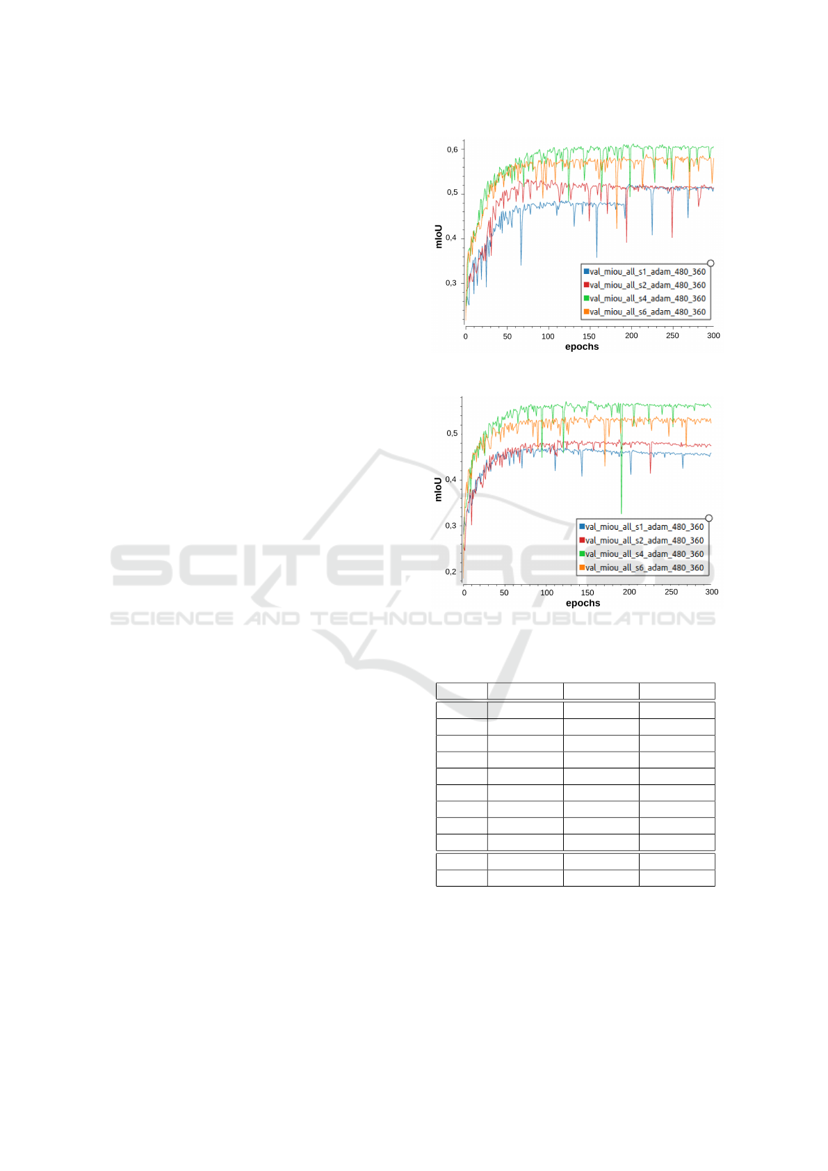
3.4 Training Results
In this paper, mean intersection over union, noted
mIoU, is used to evaluate the performance of our seg-
net models for the two datasets. The mIoU metric
measures the number of common pixels between the
label and prediction masks (i.e. intersection of the two
sets) divided by the total number of pixels present in
the two masks (i.e. union of the two sets). mIoU,
also known as the Jaccard index, is one of the most
commonly used metrics for the accuracy of semantic
segmentation models (Minaee et al., 2022). Figures 4
and 5 illustrate the evolution of the mIoU on the val-
idation set over the 300 training epochs for 4 Segnet
architectures (Segnet 1, 2, 4 and 6).
Tables 3 and 4 resume the best obtained mIoU
values for all architectures and all image resolutions.
Note that, for comparison purpose, we also train two
other famous encoder-decoder models, namely Enet
(Paszke et al., 2016) or Erfnet (Romera et al., 2018)
with the same environment as described in Section
3.3. These two models, based on more complex di-
lated and transposed convolution operations, are very
efficient and accurate (Zelek and Jeon, 2022).
Figure 4: UDD6 validation set mIoU evolution over training
epochs for Segnet 1, 2, 4 and 6 (resolution 480 × 360).
Figure 5: UAVid validation set mIoU evolution over training
epochs for Segnet 1, 2, 4 and 6 (resolution 480 × 360).
Table 3: UDD best mIoU for all architectures/resolutions.
ID 480 × 360 640 × 360 820 × 460
1 0.521 0.538 0.542
2 0.533 0.549 0.572
3 0.590 0.592 0.600
4 0.612 0.603 0.625
5 0.609 0.610 0.624
6 0.588 0.593 0.602
7 0.556 0.566 0.560
8 0.593 0.600 0.605
9 0.606 0.610 0.617
Enet 0.609 0.620 ∅
Erfnet 0.612 0.632 ∅
3.5 Analysis
Based on the results, we can observe that, overall,
the original Segnet architecture (Segnet 1) is the less
accurate one for the two validation sets. As oppo-
site, Segnet 4 seems the most accurate one followed
Exploring Segnet Architectures for iGPU Embedded Devices
423

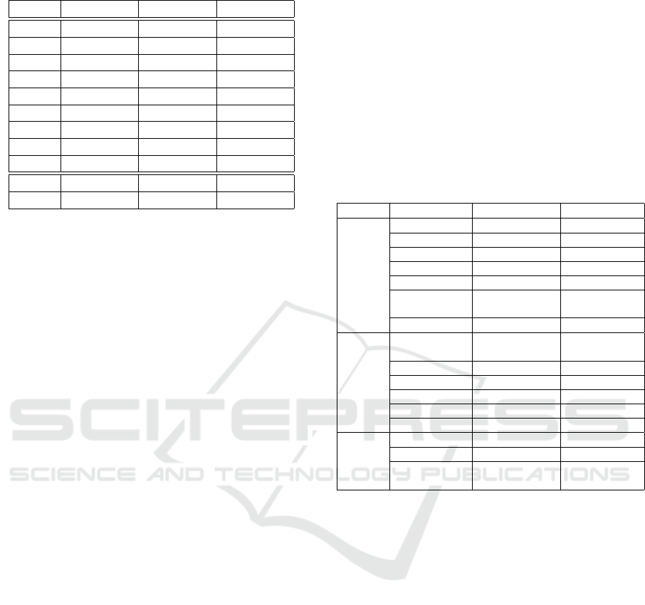
Table 4: UAVid best mIoU for all architectures/resolutions.
ID 480 × 360 640 × 360 820 × 460
1 0.473 0.491 0.519
2 0.487 0.486 0.518
3 0.538 0.552 0.576
4 0.567 0.574 0.586
5 0.565 0.574 0.590
6 0.541 0.545 0.556
7 0.529 0.537 0.540
8 0.553 0.559 0.571
9 0.563 0.567 0.586
Enet 0.541 0.552 ∅
Erfnet 0.554 0.558 ∅
closely by Segnet 5 (containing additional residual
connections) and, also, Segnet 9. The model Segnet
6 offers a good compromise, being very small, and
still offering good accuracy. We can also notice that
the use of higher resolution images, despite increas-
ing drastically the number of arithmetic operations,
improves only slightly the best mIoU value, the most
sensible to the increase of resolution are Segnet 1,2
and 3 which makes sense since these are the biggest
models in the experiments, therefore, they might be
able to capture more information from the biggest fea-
ture maps generated with higher resolution images.
Enet and Erfnet models are also providing good re-
sults similar to what is obtained for the best perform-
ing Segnet architectures. The trade-off between mod-
els mIoU accuracy and on-board execution time will
be discussed in Section 4.3. Note that due to a limi-
tation of our hardware/software settings on the devel-
opment platform, we haven’t been able to run Enet
and Erfnet models on the highest resolution training
set (820 × 460).
4 IMPLEMENTATIONS AND
RESULTS
4.1 Hardware Platform
The implementation of the Segnet architectures pro-
posed in Section 3.2 is done on the NVIDIA Jetson
AGX Orin 64 GB (NVIDIA, 2022) and NVIDIA Jet-
son Xavier NX (NVIDIA, 2020) MPSoCs:
• On the Orin, the NVIDIA Ampere Architecture
iGPU found within this SoC is used for running
the semantic segmentation model. The iGPU is
made up of 2048 CUDA cores distributed among 16
Streaming Multiprocessors (SMs). The 128 cores
in each SM share 192 KB of combined L1 cache
and shared memory and the 16 SMs share an L2
cache memory of 4 MB.
• On the Xavier NX, the Volta Architecture iGPU is
used for executing the image segmentation archi-
tecture. In this case, the iGPU has 384 CUDA cores
split between 2 SMs. Each SM has a 128 KB L1
data cache and shared memory while the 2 SMs
share 512 KB.
Table 5 summarizes the most important features
of these MPSoCs.
Table 5: NVIDIA Jetson AGX Orin 64GB and NVIDIA
Jetson Xavier NX characteristics.
AGX Orin 64GB Xavier NX
iGPU
Architecture Ampere Volta
C.C. 8.7 7.2
SM 16 2
CUDA cores 2048 384
Max freq. 1.3 GHz 1.1 GHz
L1D cache +
shared memory
192 KB 128 KB
L2 cache
4 MB 512 KB
ARM
CPU
Complex
ARMv8.2-A
cores per cluster
4 Cortex A78AE
@ 2.2 GHz
2 Nvidia Carmel
@ 1.4 GHz
Clusters 3 3
L1I cache 64 KB 128 KB
L1D cache 64 KB 64 KB
L2 cache 256 KB 2 MB per cluster
L3 cache 2 MB per cluster shared, 4 MB
System
System cache 4 MB ∅
LPDDR v5, 64 GB v4, 8 GB
SoC power
consumption
60 W 20 W
4.2 Code Optimizations
In CNNs, the convolution operation accounts for most
of the execution time, hence being object of optimiza-
tions. Traditional image convolutions (i.e. addition of
element-wise multiplications of neighbour pixels) re-
quire as many floating point operations as filter size
per image pixel. In order to reduce this arithmetical
complexity, algorithms based on data transformations
are performed, e.g. im2col + Basic Linear Algebra
Subprograms, Fast Fourier Transform, Strassen con-
volution, Winograd convolution. Winograd’s minimal
filtering algorithm, originally proposed by Winograd
for signal processing problems (Winograd, 1980), has
been then applied in deep learning applications (Lavin
and Gray, 2016). Winograd’s convolution works with
small tiles of pixels rather with one pixel at a time.
Assuming 3×3 filters, the floating point multiplica-
tion complexity with respect to traditional convolu-
tion can be reduced ×2.25 and ×4 for output tiles of
2×2 and 4×4 respectively. Note that depending on
NCTA 2023 - 15th International Conference on Neural Computation Theory and Applications
424

the tile size, a given number of additions, subtractions
and multiplications must be done for the data transfor-
mation. The filter transformations can be computed
offline as these are known beforehand. The decom-
position on linear matrices for the Winograd convolu-
tion is described in (Barabasz and Gregg, 2019) and
its implementation on GPU in (Yan et al., 2020; Cas-
tro et al., 2021).
On NVIDIA platforms, cuDNN library is often
used as reference for ANN computations due to its
performance and abstraction. Different works have
proposed their own Winograd convolution implemen-
tation that outperforms the cuDDN version they com-
pared with. These works make use of assembly code
(SSAS), compilation changes (NVCC yield flag),
kernel fusion (level kernels merged together), big-
ger Winograd tiles (Winograd 6x6) or mix-precision
floating point operations (16-bit and 32-bit) (Yan
et al., 2020; Castro et al., 2021; Liu et al., 2021).
Strassen Convolution can also be used to optimize
traditional convolution (Cong and Xiao, 2014). Nev-
ertheless, Hissan has shown that Strassen method is
very error prone especially with matrices and some
arrangements have been analyzed to get this method
safer (De Silva et al., 2018). However, Winograd fil-
tering algorithm is currently the most used convolu-
tion optimization in deep learning applications.
Our implementation of Winograd convolutions
does not consider assembly inline code, compiler
optimization, kernel fusion or floating points mix-
precision, which are left as future work. Ours makes
use of static shared memory (dynamic shared mem-
ory when required) which gives the possibility to ex-
change data among threads residing in the same block
at the L1 cache level. Shared memory also allows us
to have predictable execution times as it does not de-
pend on the L1 cache replacement policies but explic-
itly on our code. Convolution operations, bias convo-
lution addition and batch normalization (when appli-
cable) are performed in the same CUDA kernel. Up-
sampling and downsampling operations are executed
in separated kernels.
4.3 Results and Discussion
The Segnet architectures considered for implementa-
tions are 1, 2, 3, 4, 6 and 9 (see Table 1). Architecture
5 is discarded as residual connections weren’t pro-
viding significant mIoU improvements compared to
non-residual Segnet 4 as shown in Section 3.4. Sim-
ilarly, Segnet 7 and 8 are not considered as they did
not offer satisfying mIoU accuracy versus model size
compromise with respect to other architectures such
as 4, 6 or 9. For the sake of comparison, convolu-
tions are performed in different ways for the consid-
ered architectures: (I) Traditional, (II) 2×2 output tile
Winograd and (III) 4×4 output tile Winograd. The
filter weights transformation required by the Wino-
grad convolutions are precomputed. In addition, we
consider two modes according to the batch normal-
ization integration: (A) not integrated, i.e. the nor-
malization is applied online and (B) integrated, i.e.
the normalization is already included within the filter
weights. We only contemplate 3×3 filters and 32-bit
floats. Table 6 shows the measured Worst-Case Exe-
cution Time (WCET), Average-Case Execution Time
(ACET), the Best-Case Execution Time (BCET) and
the time VARiance (VAR) when performing the ex-
periments on the Orin SoC. The execution time of the
different Segnet architectures are measured through
CUDA events recording (elapsed time of the start and
finish events). The measured time includes the ini-
tial input image resize from 3840 × 2160 or 4096 ×
2160 to 480 × 430, 640 × 360 or 820 × 460, the Seg-
net execution and the image coloring. A total of 1000
measurements are taken.
In terms of Segnet architecture, Segnet 6 is the
fastest from all of them due to the reduced number of
levels, and especially, of number of output channels.
Furthermore, it offers the lowest variability (VAR),
which can be explained by its low WCET-ACET and
ACET-BCET difference. The architecture with the
highest mIoU (i.e. Segnet 4) offers slightly worse re-
sults than Segnet 3, being these two slower than Seg-
net 2, 6 and 9. The original Segnet architecture (i.e.
Segnet 1), is the slowest from all of them, and as seen
in Section 4.1, its mIoU is the worst. Therefore, this
architecture becomes dominated by other Segnet ar-
chitectures.
In respect of the type of convolution, the 4×4 out-
put Winograd (configuration III) is the fastest as ex-
pected. Using the traditional convolution (configura-
tion I) as reference and considering all the implemen-
tations, configurations II and III provide an average
ACET performance boost of ×2.23 and ×2.43 respec-
tively. The fact that configuration II offers practical
performance similar to the theoretical value (×2.25
time reduction) can be as a consequence of a more
optimal CUDA convolution implementation after re-
writing the CUDA kernel code for Winograd. Overall,
Winograd 4×4 does not seem to hugely improve the
execution time with respect to Winograd 2×2. Cu-
riously, for Segnet 9, Winograd 4×4 is slower than
Winograd 2×2. In order to understand why Wino-
grad 4×4 is far for its theoretical improvement with
respect to the traditional convolution (×4 time reduc-
tion), experiments were also conducted on the Xavier
NX SoC. The Winograd 2×2 and Winograd 4×4 re-
Exploring Segnet Architectures for iGPU Embedded Devices
425

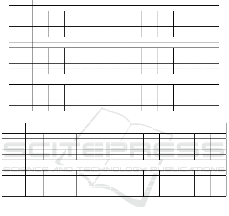
Table 6: Metrics of different Segnet architectures execution on Jetson AGX Orin 64GB for an input image of 480x360.
I: Traditional Convolution
A: Non-integrated Normalization B: Integrated Normalization
Architecture 1 2 3 4 6 9 1 2 3 4 6 9
WCET (ms) 500.41 154.69 315.19 318.41 85.38 204.85 495.95 151.45 316.74 316.29 84.34 201.48
ACET (ms) 490.67 149.06 312.78 315.92 84.06 203.13 487.79 149.45 313.25 312.83 83.11 200.12
BCET (ms) 482.59 146.88 310.34 313.98 83.86 202.56 480.78 147.16 310.81 310.88 82.96 199.60
VAR (msˆ2) 7.41 0.43 0.66 0.45 0.01 0.04 6.50 0.42 0.81 0.57 0.00 0.03
II: Winograd 2×2
A: Non-integrated Normalization B: Integrated Normalization
Architecture 1 2 3 4 6 9 1 2 3 4 6 9
WCET (ms) 237.71 70.42 143.35 144.81 35.89 91.19 240.57 70.06 144.08 144.57 36.86 90.23
ACET (ms) 230.51 67.54 140.49 142.08 35.53 89.70 232.38 67.11 141.29 141.85 35.54 88.60
BCET (ms) 221.39 64.25 138.21 139.79 35.34 88.62 224.53 64.01 138.48 139.52 35.20 87.11
VAR (msˆ2) 7.21 1.06 0.74 0.62 0.00 0.18 4.88 1.27 0.76 0.58 0.01 0.28
III: Winograd 4×4
A: Non-integrated Normalization B: Integrated Normalization
Architecture 1 2 3 4 6 9 1 2 3 4 6 9
WCET (ms) 196.95 58.68 132.17 134.96 32.24 96.14 196.56 60.13 133.33 136.02 32.63 94.83
ACET (ms) 195.29 57.70 130.75 133.60 32.06 94.90 195.02 58.84 132.22 134.65 31.40 93.51
BCET (ms) 168.90 57.25 129.50 132.27 31.90 94.35 170.68 58.47 131.15 133.70 31.20 93.09
VAR (msˆ2) 0.93 0.02 0.20 0.19 0.00 0.03 0.74 0.01 0.11 0.11 0.00 0.02
Table 7: Metrics of different Segnet architectures execution on Jetson Xavier NX for an input image of 480x360.
II: Winograd 2×2
A: Non-integrated Normalization B: Integrated Normalization
Architecture 1 2 3 4 6 9 1 2 3 4 6 9
WCET (ms) 1800.33 474.70 1450.33 1434.90 238.38 836.24 1736.64 470.05 1429.59 1406.98 237.84 810.60
ACET (ms) 1732.36 453.55 1412.24 1403.56 234.81 821.45 1700.06 454.05 1394.93 1374.48 235.27 797.30
BCET (ms) 1687.50 434.76 1360.21 1361.66 231.45 807.81 1662.02 432.86 1349.20 1336.01 233.72 788.42
VAR (msˆ2) 289.10 61.07 224.94 182.44 1.34 33.28 189.73 47.60 207.68 156.85 0.57 13.05
III: Winograd 4×4
A: Non-integrated Normalization B: Integrated Normalization
Architecture 1 2 3 4 6 9 1 2 3 4 6 9
WCET (ms) 1026.32 289.60 697.12 799.78 174.74 625.34 1000.08 276.12 673.93 768.84 159.51 559.59
ACET (ms) 1007.22 283.44 684.66 784.58 171.67 612.87 966.19 266.93 646.48 736.84 153.54 535.88
BCET (ms) 903.41 276.78 677.30 775.07 167.59 601.11 853.16 260.69 625.68 716.76 148.56 516.37
VAR (msˆ2) 91.17 5.04 12.34 13.11 2.11 18.54 131.71 9.38 60.16 77.96 3.49 49.71
sults can be seen in Table 7. On this SoC, we can ap-
preciate the benefit of using Winograd 4×4, obtaining
a ×1.7 ACET gain on average with respect to Wino-
grad 2×2 when considering all the architectures. This
means that the iGPU architecture also affects the ef-
fectiveness of Winograd convolutions. The execution
time of these Segnet architectures varies significantly
less on the Orin SoC. In addition, the use of Wino-
grad 4×4 reduces the variability value independently
of the architecture.
Regarding the normalization integration in the fil-
ter weights on both SoCs, the vast majority of the
architectures have execution gains (e.g. Segnet 6.III
or 9.III) while others become unaffected (e.g. Segnet
4.III on the Xavier NX or 3.III on the Orin). The lat-
ter occurs due to CUDA compilation behaviors which
should be treated specifically for the given Segnet ar-
chitecture. Overall, the use of integrated batch nor-
malization saves 16.98 ms and 39.77 ms of ACET
for Winograd 2×2 and 4×4 respectively when con-
sidering all the Segnet architectures. It must be noted
that the integrated normalization configuration only
performs a bias convolution addition unlike the non-
integrated configuration, and thus saving 1 subtrac-
tion, 1 addition, 1 multiplication, 1 division and 1
square root operations. The effect of the input im-
age resolution on the execution of the proposed Seg-
net architectures is also studied. The resolutions to
use are those mentioned in Section 3.3, i.e. 480 ×
360, 640 × 360 and 820 × 460. The results on the
Jetson AGX Orin can be seen in Table 8. Indepen-
dently of the convolution type, the increase of execu-
tion time as function of the input image resolution can
be assumed to be linear, e.g. moving from 480 × 360
to 820 × 460 (×2.183 pixels) for Segnet 6 with con-
figurations I.B, II.B and III.B we observe a ×2.185,
NCTA 2023 - 15th International Conference on Neural Computation Theory and Applications
426

×2.135 and ×2.189 increase respectively.
To visualize which Segnet architectures are dom-
inant for the used datasets, Figures 6 and 7 show the
mIoU-performance trade-off for each Segnet architec-
ture when using configuration III.B for the UDD6 and
UAVid datasets respectively. The tag ID refers to the
Segnet architecture and the R to the input image res-
olution (R1, R2 and R3 are 480 × 360, 640 × 360
and 820 × 460 respectively). Red marks are dom-
inated Segnet architectures while those in green are
non-dominated architectures. For the UDD6 dataset,
Segnet 1 (original Segnet), 2 and 3 are always dom-
inated by Segnet 4 (except resolution 640 × 360), 6
and 9. The UAVid dataset has similar results, being
Segnet 6 and 9 the dominant architectures. These re-
sults show that, in our experiments, Segnet architec-
tures with 3 levels are more suitable than those with
4 and 5 in terms of accuracy, which might come from
the noise introduced during the learning process due
to spatial resolution reduction (pooling).
ID 1, R1
ID 1, R2
ID 1, R3
ID 2, R1
ID 2, R2
ID 2, R3
ID 3, R1
ID 4, R1
ID 4, R2
ID 4, R3
ID 6, R1
ID 6, R2
ID 6, R3
ID 8, R1
ID 8, R2
ID 8, R3
ID 9, R1
ID 9, R2
ID 9, R3
0
50
100
150
200
250
300
350
400
450
0,52 0,54 0,56 0,58 0,60 0,62 0,64
ACET (MS)
MIOU
Dominated Segnet architecture
Non-dominated Segnet architecture
Figure 6: III.B UDD6 ACET-mIoU trade-off on Jetson
Orin.
ID 1, R1
ID 1, R2
ID 1, R3
ID 2, R1
ID 2, R2
ID 2, R3
ID 3, R1
ID 4, R1
ID 4, R2
ID 4, R3
ID 6, R1
ID 6, R2
ID 6, R3
ID 8, R1
ID 8, R2
ID 8, R3
ID 9, R1
ID 9, R2
ID 9, R3
0
50
100
150
200
250
300
350
400
450
0,46 0,48 0,5 0,52 0,54 0,56 0,58 0,6
ACET (MS)
MIOU
Dominated Segnet architecture
Non-dominated Segnet architecture
Figure 7: III.B UAVid ACET-mIoU trade-off on Jetson
Orin.
5 CONCLUSION AND
PERSPECTIVES
In this paper, we have investigated 8 architectures
based on the original Segnet. We have provided a
complete analysis and have shown that, for our ex-
periments based on UDD6 and UAVid datasets, the
original Segnet model is not the most optimal one de-
spite being the biggest one. The most accurate ac-
cording to mIoU metric is Segnet 4 followed closely
by Segnet 9. Segnet 6 offers a very good compro-
mise and achieve correct on-board performance for
a proper accuracy. This architecture, using our im-
plementation, is capable to ensure 30 Hz execution
frequency on the Jetson Orin and 5 Hz on the Jetson
Xavier NX. Parts of the presented results can be re-
produced as we have released the major part of our
code as an open-source package containing Pytorch
training environment, CUDA implementation as well as
the models binaries to reproduce our results
4
.
Many perspectives are possible to follow up this
work. First, we can investigate other options to opti-
mize training like the use schedule for learning rates,
weights decays or other optimizers in order to get
more accurate models. Secondly, another interesting
topic can be to combine RNN concepts such as Con-
vLSTM (Shi et al., 2015) into our Segnet 4, 6 or 9
architectures to extract properly the temporal relation
in the image sequences of UAVID dataset and, there-
fore, being capable of distinguish the moving car from
static car. From the real-time implementation point
of view, we plan to investigate the use of fixed point
arithmetic, explore the CUDA tensor cores and look
into L2 cache memory locking policy. In addition,
from this baseline, we want to follow up on our imple-
mentation and extend it to more complex structures
with dilated convolutions and transposed convolution
such as Enet (Paszke et al., 2016) or Erfnet (Romera
et al., 2018) by integrating more recent Winograd op-
timizations (Kim et al., 2019; Yepez and Ko, 2020).
ACKNOWLEDGEMENTS
This work was supported by the Defense Innova-
tion Agency (AID) of the French Ministry of De-
fense (research project CONCORDE N° 2019 65
0090004707501).
4
https://github.com/ISAE-PRISE/gpu4seg
Exploring Segnet Architectures for iGPU Embedded Devices
427

Table 8: Metrics of 3 Segnet architectures execution on Jetson AGX Orin 64GB for different input image resolutions.
I.B: Traditional Convolution - Integrated
Architecture
Resolution
1
480×360
1
640×360
1
820×460
4
480×360
4
640×360
4
820×460
6
480×360
6
640×360
6
820×460
WCET (ms) 495.95 660.97 1084.84 316.29 417.40 681.96 84.34 112.26 183.13
ACET (ms) 487.79 649.40 1068.55 312.83 414.97 678.47 83.11 110.82 181.57
BCET (ms) 480.78 639.20 1046.08 310.88 412.69 676.04 82.96 110.65 181.37
VAR (msˆ2) 6.50 13.36 30.40 0.57 0.56 0.82 0.00 0.01 0.01
II.B: Winograd 2×2 - Integrated
Architecture
Resolution
1
480×360
1
640×360
1
820×460
4
480×360
4
640×360
4
820×460
6
480×360
6
640×360
6
820×460
WCET (ms) 240.57 319.95 527.47 144.57 196.73 320.62 36.86 47.31 77.15
ACET (ms) 232.38 310.04 515.06 141.85 191.29 314.53 35.54 46.73 75.89
BCET (ms) 224.53 299.57 503.58 139.52 187.33 309.23 35.20 46.45 75.48
VAR (msˆ2) 4.88 9.64 17.21 0.58 1.52 3.56 0.01 0.02 0.03
III.B: Winograd 4×4 - Integrated
Architecture
Resolution
1
480×360
1
640×360
1
820×460
4
480×360
4
640×360
4
820×460
6
480×360
6
640×360
6
820×460
WCET (ms) 196.56 261.15 421.78 136.02 183.67 302.17 32.63 42.03 69.84
ACET (ms) 195.02 258.93 417.50 134.65 180.88 296.74 31.40 41.81 68.73
BCET (ms) 170.68 227.02 366.63 133.70 179.56 294.70 31.20 41.61 68.43
VAR (msˆ2) 0.74 1.38 4.08 0.11 0.21 0.65 0.00 0.00 0.01
REFERENCES
Amert, T., Otterness, N., Yang, M., Anderson, J. H., and
Smith, F. D. (2017). Gpu scheduling on the nvidia
tx2: Hidden details revealed. In 2017 IEEE Real-Time
Systems Symposium (RTSS), pages 104–115.
Badrinarayanan, V., Kendall, A., and Cipolla, R. (2017).
Segnet: A deep convolutional encoder-decoder ar-
chitecture for image segmentation. IEEE Transac-
tions on Pattern Analysis and Machine Intelligence,
39(12):2481–2495.
Barabasz, B. and Gregg, D. (2019). Winograd convolu-
tion for dnns: Beyond linear polynomials. In Alviano,
M., Greco, G., and Scarcello, F., editors, AI*IA 2019
– Advances in Artificial Intelligence, pages 307–320,
Cham. Springer International Publishing.
Canny, J. (1986). A computational approach to edge de-
tection. IEEE Transactions on Pattern Analysis and
Machine Intelligence, PAMI-8(6):679–698.
Castro, R. L., Andrade, D., and Fraguela, B. B. (2021).
Opencnn: A winograd minimal filtering algorithm im-
plementation in cuda. Mathematics, 9(17).
Chen, Y., Wang, Y., Lu, P., Chen, Y., and Wang, G. (2018).
Large-scale structure from motion with semantic con-
straints of aerial images. In Lai, J.-H., Liu, C.-L.,
Chen, X., Zhou, J., Tan, T., Zheng, N., and Zha,
H., editors, Pattern Recognition and Computer Vision,
pages 347–359, Cham. Springer International Pub-
lishing.
Chetlur, S., Woolley, C., Vandermersch, P., Cohen, J.,
Tran, J., Catanzaro, B., and Shelhamer, E. (2014).
cudnn: Efficient primitives for deep learning. CoRR,
abs/1410.0759.
Cong, J. and Xiao, B. (2014). Minimizing computation in
convolutional neural networks. In Wermter, S., We-
ber, C., Duch, W., Honkela, T., Koprinkova-Hristova,
P., Magg, S., Palm, G., and Villa, A. E. P., editors,
Artificial Neural Networks and Machine Learning –
ICANN 2014, pages 281–290, Cham. Springer Inter-
national Publishing.
De Silva, H., Gustafson, J. L., and Wong, W.-F. (2018).
Making strassen matrix multiplication safe. In 2018
IEEE 25th International Conference on High Perfor-
mance Computing (HiPC), pages 173–182.
Deravi, F. and Pal, S. (1983). Grey level thresholding using
second-order statistics. Pattern Recognition Letters,
1(5):417–422.
Dhanachandra, N., Manglem, K., and Chanu, Y. J. (2015).
Image segmentation using k-means clustering algo-
rithm and subtractive clustering algorithm. Procedia
Computer Science, 54:764–771.
Fukushima, K. (1980). Neocognitron: A self-organizing
neural network model for a mechanism of pattern
recognition unaffected by shift in position. Biologi-
cal Cybernetics, 36:193–202.
Hatcher, W. G. and Yu, W. (2018). A survey of deep learn-
ing: Platforms, applications and emerging research
trends. IEEE Access, 6:24411–24432.
He, K., Zhang, X., Ren, S., and Sun, J. (2015). Delving
deep into rectifiers: Surpassing human-level perfor-
mance on imagenet classification. In 2015 IEEE In-
ternational Conference on Computer Vision (ICCV),
pages 1026–1034.
He, K., Zhang, X., Ren, S., and Sun, J. (2016). Deep resid-
ual learning for image recognition. In 2016 IEEE Con-
ference on Computer Vision and Pattern Recognition
(CVPR), pages 770–778.
Hirahara, D., Takaya, E., Kobayashi, Y., and Ueda, T.
(2021). Effect of the pixel interpolation method for
downsampling medical images on deep learning ac-
NCTA 2023 - 15th International Conference on Neural Computation Theory and Applications
428

curacy. Journal of Computer and Communications,
9:150–156.
Ioffe, S. and Szegedy, C. (2015). Batch normalization: Ac-
celerating deep network training by reducing inter-
nal covariate shift. In Proceedings of the 32nd In-
ternational Conference on International Conference
on Machine Learning - Volume 37, ICML’15, page
448–456. JMLR.org.
Irie and Miyake (1988). Capabilities of three-layered per-
ceptrons. In IEEE 1988 International Conference on
Neural Networks, pages 641–648 vol.1.
Jeong, E., Kim, J., and Ha, S. (2022). Tensorrt-based frame-
work and optimization methodology for deep learning
inference on jetson boards. ACM Transactions on Em-
bedded Computing Systems, 21(5).
Kanopoulos, N., Vasanthavada, N., and Baker, R. (1988).
Design of an image edge detection filter using the so-
bel operator. IEEE Journal of Solid-State Circuits,
23(2):358–367.
Kim, M., Park, C., Kim, S., Hong, T., and Ro, W. W.
(2019). Efficient dilated-winograd convolutional neu-
ral networks. In 2019 IEEE International Conference
on Image Processing (ICIP), pages 2711–2715.
Kingma, D. P. and Ba, J. (2015). Adam: A method for
stochastic optimization. In Bengio, Y. and LeCun,
Y., editors, 3rd International Conference on Learn-
ing Representations, ICLR 2015, San Diego, CA, USA,
May 7-9, 2015, Conference Track Proceedings.
Krizhevsky, A., Sutskever, I., and Hinton, G. E. (2012).
Imagenet classification with deep convolutional neu-
ral networks. In Pereira, F., Burges, C., Bottou, L.,
and Weinberger, K., editors, Advances in Neural In-
formation Processing Systems, volume 25. Curran As-
sociates, Inc.
Lavin, A. and Gray, S. (2016). Fast algorithms for convo-
lutional neural networks. In 2016 IEEE Conference
on Computer Vision and Pattern Recognition (CVPR),
pages 4013–4021.
Lecun, Y., Bottou, L., Bengio, Y., and Haffner, P. (1998).
Gradient-based learning applied to document recogni-
tion. Proceedings of the IEEE, 86(11):2278–2324.
Lee, M., Kim, M., and Jeong, C. Y. (2022). Real-time se-
mantic segmentation on edge devices: A performance
comparison of segmentation models. In 2022 13th In-
ternational Conference on Information and Commu-
nication Technology Convergence (ICTC), pages 383–
388.
Lin, T.-Y., Doll
´
ar, P., Girshick, R., He, K., Hariharan, B.,
and Belongie, S. (2017). Feature pyramid networks
for object detection. In 2017 IEEE Conference on
Computer Vision and Pattern Recognition (CVPR),
pages 936–944.
Liu, J., Yang, D., and Lai, J. (2021). Optimizing winograd-
based convolution with tensor cores. In Proceedings
of the 50th International Conference on Parallel Pro-
cessing, ICPP ’21, New York, NY, USA. Association
for Computing Machinery.
Liu, S. and Deng, W. (2015). Very deep convolutional
neural network based image classification using small
training sample size. In 2015 3rd IAPR Asian Confer-
ence on Pattern Recognition (ACPR), pages 730–734.
Long, J., Shelhamer, E., and Darrell, T. (2015). Fully con-
volutional networks for semantic segmentation. In
2015 IEEE Conference on Computer Vision and Pat-
tern Recognition (CVPR), pages 3431–3440.
Lyu, Y., Vosselman, G., Xia, G.-S., Yilmaz, A., and Yang,
M. Y. (2020). Uavid: A semantic segmentation dataset
for uav imagery. ISPRS Journal of Photogrammetry
and Remote Sensing, 165:108–119.
Mahony, N. O., Campbell, S., Carvalho, A., Harapanahalli,
S., Velasco-Hern
´
andez, G. A., Krpalkova, L., Riordan,
D., and Walsh, J. (2019). Deep learning vs. traditional
computer vision. In Computer Vision Conference.
Minaee, S., Boykov, Y., Porikli, F., Plaza, A., Kehtarnavaz,
N., and Terzopoulos, D. (2022). Image segmenta-
tion using deep learning: A survey. IEEE Transac-
tions on Pattern Analysis and Machine Intelligence,
44(7):3523–3542.
Neves, G. F., Chaudron, J.-B., and Dion, A. (2021). Recur-
rent neural networks analysis for embedded systems.
In NCTA 2021 - 13th International Joint Conference
on Neural Computation Theory and Applications, Vir-
tual Event, FR.
Noh, H., Hong, S., and Han, B. (2015). Learning decon-
volution network for semantic segmentation. In 2015
IEEE International Conference on Computer Vision
(ICCV), pages 1520–1528, Los Alamitos, CA, USA.
IEEE Computer Society.
NVIDIA (2020). NVIDIA Xavier Series System-on-Chip -
TECHNICAL REFERENCE MANUAL.
NVIDIA (2022). NVIDIA Orin Series System-on-Chip -
TECHNICAL REFERENCE MANUAL.
NVIDIA (2023). Ampere Tuning Guide.
Osco, L., Junior, J., Ramos, A. P., Jorge, L., Fatholahi, S. N.,
Silva, J., Matsubara, E., Pistori, H., Gonc¸alves, W.,
and Li, J. (2021). A review on deep learning in uav re-
mote sensing. International Journal of Applied Earth
Observation and Geoinformation, 102:102456.
Otsu, N. (1979). A threshold selection method from gray-
level histograms. IEEE Transactions on Systems,
Man, and Cybernetics, 9(1):62–66.
Paszke, A., Chaurasia, A., Kim, S., and Culurciello, E.
(2016). Enet: A deep neural network architecture for
real-time semantic segmentation.
Paszke, A., Gross, S., Massa, F., Lerer, A., Bradbury, J.,
Chanan, G., Killeen, T., Lin, Z., Gimelshein, N.,
Antiga, L., Desmaison, A., K
¨
opf, A., Yang, E. Z.,
DeVito, Z., Raison, M., Tejani, A., Chilamkurthy, S.,
Steiner, B., Fang, L., Bai, J., and Chintala, S. (2019).
Pytorch: An imperative style, high-performance deep
learning library. CoRR, abs/1912.01703.
Perez-Cerrolaza, J., Abella, J., Kosmidis, L., Calderon,
A. J., Cazorla, F., and Flores, J. L. (2022). Gpu de-
vices for safety-critical systems: A survey. ACM Com-
puting Surveys, 55(7).
Romera, E.,
´
Alvarez, J. M., Bergasa, L. M., and Ar-
royo, R. (2018). Erfnet: Efficient residual factorized
convnet for real-time semantic segmentation. IEEE
Exploring Segnet Architectures for iGPU Embedded Devices
429

Transactions on Intelligent Transportation Systems,
19(1):263–272.
Ronneberger, O., Fischer, P., and Brox, T. (2015). U-
net: Convolutional networks for biomedical image
segmentation. In Navab, N., Hornegger, J., Wells,
W. M., and Frangi, A. F., editors, Medical Image Com-
puting and Computer-Assisted Intervention – MICCAI
2015, pages 234–241, Cham. Springer International
Publishing.
Rosenblatt, F. (1957). The Perceptron - A Perceiving and
Recognizing Automaton. Technical Report 85-460-1,
Cornell Aeronautical Laboratory.
Rumelhart, D. E. and McClelland, J. L. (1987). Learning
Internal Representations by Error Propagation, pages
318–362.
Russakovsky, O., Deng, J., Su, H., Krause, J., Satheesh,
S., Ma, S., Huang, Z., Karpathy, A., Khosla, A.,
Bernstein, M., Berg, A. C., and Fei-Fei, L. (2015).
ImageNet Large Scale Visual Recognition Challenge.
International Journal of Computer Vision (IJCV),
115(3):211–252.
Shi, X., Chen, Z., Wang, H., Yeung, D.-Y., Wong, W.-k.,
and Woo, W.-c. (2015). Convolutional lstm network:
A machine learning approach for precipitation now-
casting. NIPS’15, page 802–810, Cambridge, MA,
USA. MIT Press.
Sli
ˇ
z, J. and Mikulka, J. (2016). Advanced image segmenta-
tion methods using partial differential equations: A
concise comparison. In 2016 Progress in Electro-
magnetic Research Symposium (PIERS), pages 1809–
1812.
Strigl, D., Kofler, K., and Podlipnig, S. (2010). Performance
and scalability of gpu-based convolutional neural net-
works. In 2010 18th Euromicro Conference on Paral-
lel, Distributed and Network-based Processing, pages
317–324.
Winograd, S. (1980). Arithmetic Complexity of Computa-
tions. Society for Industrial and Applied Mathemat-
ics.
Yam, Y. and Chow, T. (1993). Extended backpropagation
algorithm. Electronics Letters, 29:1701–1702(1).
Yan, D., Wang, W., and Chu, X. (2020). Optimizing batched
winograd convolution on gpus. In Proceedings of the
25th ACM SIGPLAN Symposium on Principles and
Practice of Parallel Programming, PPoPP ’20, page
32–44, New York, NY, USA. Association for Com-
puting Machinery.
Yang, M., Otterness, N., Amert, T., Bakita, J., Anderson,
J. H., and Smith, F. D. (2018). Avoiding pitfalls when
using NVIDIA gpus for real-time tasks in autonomous
systems. In Altmeyer, S., editor, 30th Euromicro Con-
ference on Real-Time Systems, ECRTS 2018, July 3-6,
2018, Barcelona, Spain, volume 106 of LIPIcs, pages
20:1–20:21. Schloss Dagstuhl - Leibniz-Zentrum f
¨
ur
Informatik.
Yepez, J. and Ko, S.-B. (2020). Stride 2 1-d, 2-d, and 3-
d winograd for convolutional neural networks. IEEE
Transactions on Very Large Scale Integration (VLSI)
Systems, 28(4):853–863.
Zaitoun, N. M. and Aqel, M. J. (2015). Survey on im-
age segmentation techniques. Procedia Computer Sci-
ence, 65:797–806. International Conference on Com-
munications, management, and Information technol-
ogy (ICCMIT’2015).
Zelek, R. and Jeon, H. (2022). Characterization of se-
mantic segmentation models on mobile platforms for
self-navigation in disaster-struck zones. IEEE Access,
10:73388–73402.
Zhao, H., Shi, J., Qi, X., Wang, X., and Jia, J. (2017). Pyra-
mid scene parsing network. In 2017 IEEE Conference
on Computer Vision and Pattern Recognition (CVPR),
pages 6230–6239.
NCTA 2023 - 15th International Conference on Neural Computation Theory and Applications
430