Curved Surface Inspection by a Climbing Robot:

Path Planning Approach for Aircraft Applications

Silya Achat, Julien Marzat and Julien Moras

DTIS, ONERA, Universit

e Paris Saclay, F-91123 Palaiseau, France

Keywords:

Coverage Path Planning, Cell Decomposition, Curved Surface Inspection, Sensor Constrained Inspection.

Abstract:

This paper presents a path planning method for a climbing robot used for the exterior inspection of an aircraft.

The objective is to plan a covering path with the least possible overlap, while respecting constraints related

to an embedded sensor, a power cable, and the robot mechanical efforts. To achieve this, a semantic 2D grid

model of the aircraft is ﬁrst created by unfolding and labeling a 3D mesh reference model. An obstacle-based

area decomposition method is then applied to divide this 2D discrete space into inspection areas. Inspection

segments that satisfy the sensor constraints are then sampled and rearranged based on the order of the areas.

The connections between the inspection segments are ﬁnally determined by a weighted A

∗

search approach,

so as to limit the gravity-induced mechanical efforts on the robot.

1 INTRODUCTION

Aircraft maintenance is crucial to ensure passenger

safety, which includes inspecting their external sur-

faces to trigger condition-based maintenance opera-

tions. Early detection of defects, especially on the

fuselage, is necessary to prevent them from causing

further damage to the structure. These operations are

generally carried out manually by operators, but in re-

cent years the use of remotely operated robotic means

has been studied, in particular unmanned aerial vehi-

cles (Bugaj et al., 2020). They allow the fast observa-

tion of areas that are difﬁcult to access, while reducing

the risks taken by technicians. However, these aerial

platforms present some drawbacks. First, they require

skilled pilots which limits their development and the

use of ﬂeets. Second, they cannot deploy all types of

measurement payloads, in particular those requiring

proximity such as ultrasound measurements. Finally,

they present a risk of damage to the inspected aircraft

in case of control loss.

The use of autonomous climbing robots represents

an alternative to avoid these issues (Fernandez et al.,

2016). Indeed, by moving directly on the surface of

the aircraft, these robots will be able to conduct dif-

ferent types of observation (visual, sonar, etc.) while

not requiring a qualiﬁed pilot. Different locomotion

and adherence technologies can be considered such

as wheeled robots with ducted fans (Qin et al., 2022;

Andrikopoulos et al., 2019) or pneumatic legged con-

ﬁgurations (Wang et al., 2019), however magnetic

wheels (Starbuck et al., 2021) are not applicable for

aircraft surfaces. These climbing robots are generally

quite slow, therefore a critical point is to optimize the

inspection path allowing to cover the area so that it

is the shortest, while taking into account the inspec-

tion constraints of the embedded sensors (in range

and direction of observation), the motion of the robot

(mechanical constraint of adherence or winding of a

power cable) and prohibited areas such as the ﬁns.

This paper presents the deﬁnition of a method for

planning the inspection path for such climbing robots

to inspect the fuselage of an aircraft, considering nu-

merous operational and technical constraints. The nu-

merical performances of the procedure are evaluated

on a 3D mesh model, as illustrated in Figure 1. This

new method relies on a decomposition in areas delim-

ited by obstacles of arbitrary shapes from an unfolded

2D grid model. Inspection segments are deﬁned in

these areas with sensor constraints taken into account,

and are ﬁnally connected using a weighted A

∗

procedure to provide the global inspection path.

2 RELATED WORK

Numerous studies have addressed the problem of

computing a covering path for applications such as

surface inspection (Wu et al., 2015; Liu et al., 2022),

as well as in the context of autonomous vacuums

Achat, S., Marzat, J. and Moras, J.

Curved Surface Inspection by a Climbing Robot: Path Planning Approach for Aircraft Applications.

DOI: 10.5220/0012185300003543

In Proceedings of the 20th International Conference on Informatics in Control, Automation and Robotics (ICINCO 2023) - Volume 1, pages 433-443

ISBN: 978-989-758-670-5; ISSN: 2184-2809

433

Figure 1: Illustration of a path planned for a climbing robot

performing aircraft fuselage inspection.

(Hasan et al., 2014), industrial painting robots (Wu

and Tang, 2023; Chen et al., 2008), or problems

related to the traveling salesman (Rai et al., 2014;

Dahiya and Sangwan, 2018). These paths can be com-

puted on ﬂat or curved surfaces. In the case of curved

surfaces, there are two possible approaches: either a

path is directly computed in the 3D space based on a

3D model, or a representative 2D parametrization is

ﬁrst extracted from the 3D model to exploit a planar

model for path planning.

Various strategies can be applied to obtain a

path that fully covers the surface to be inspected.

Sampling-based methods generate random paths,

leading after many iterations to the complete scan-

ning of a given area (S

orme and Edwards, 2018). On

the other hand, deterministic methods can be more

time-efﬁcient by dividing the area of interest into sub-

areas delimited by obstacles, called cells. This section

presents a state of the art of the methods related to the

above-mentioned issues, namely path planning meth-

ods of 3D structures, different methods for construct-

ing a representative 2D model from a 3D one, and

previous works dealing with the decomposition of a

zone into sub-areas from obstacles.

Some techniques bypass the 2D representation of

space and allow for the construction of covering paths

directly on the curved surfaces to be treated. This is

the case in the work presented in (Mineo et al., 2017)

where parallel paths are calculated on the surface of a

3D mesh model of a curved piece to be followed by a

painting robot. The objective is to create paths spaced

by a constant distance d from an edge of the piece.

Planes Π

are deﬁned to be perpendicular to the refer-

ence edge, containing regularly spaced points P

. To

ﬁnd the points located at a distance d from the refer-

ence edge, we have to simply move from P

towards

the successive intersection points with a mesh of the

surface: the curvilinear distance between P

and an

intersection point is the sum of the distances between

each intersection point. The point on plane Π

at a dis-

tance d from P

is determined by linear interpolation

between the two successive intersection points having

curvilinear distances from P

respectively greater and

lower than d.

Studies on the inspection of large metallic struc-

tures such as ship hulls by small differential-drive

robots with magnetic wheels (Starbuck et al., 2021)

have focused on establishing a planar model repre-

sentative of a cylinder by stereographic projection.

This model has the advantage of being continuous and

therefore exploitable for state estimation by a Mani-

fold Invariant Extended Kalman Filter. Indeed, an un-

rolled model in cylindrical coordinates would present

a discontinuity at the angular position ±π. However,

in the context of planning an inspection path, this

kind of cylindrical parametrization would be more ap-

propriate as it involves less deformation of distances

between points on the surface. Moreover, this dis-

continuity of the unrolled model could be exploited

to manage directly the non-winding constraint of a

robot’s power cable during path planning.

Coverage Path Planning (CPP) is a well-known

discipline, and a relevant state-of-the-art is presented

in (Galceran and Carreras, 2013). A common ﬁrst

step among the methods described is the decompo-

sition of space into cells deﬁned by the obstacles

present in the space. The Boustrophedon Decom-

position method (Choset and Pignon, 1998) divides

a continuous space into cells based on the vertices

of the obstacles, which requires the obstacles to be

modeled as polygons. This constraint is lifted by

the Morse-Based Boustrophedon Cellular Decompo-

sition method (Acar et al., 2002), which deﬁnes cells

based on critical points on the obstacles depending

on the inspection direction. Other methods exploit

a discrete environment model represented as a grid,

such as the Grid Based Coverage using wavefront al-

gorithm (Zelinsky et al., 1993) and Spiral Spanning-

Tree Coverage (Gabriely and Rimon, 2001).

The method described in (Zelinsky et al., 1993)

decomposes the space into a grid of uniform cells,

where those in contact with an obstacle are not con-

sidered by the path planning algorithm. The starting

and ending cells are deﬁned, and the algorithm begins

the path search from the ending cell. The idea is to

propagate a wave from the ending cell to the starting

cell, assigning each encountered cell its distance from

the ending point. Thus, the cell at the ending point

is assigned the index 0. Then, at each iteration, this

index is incremented and assigned to all neighboring

cells that have not yet been visited. The process is

iterated until the starting cell is reached. A covering

path is then derived by starting at the starting cell and

moving at each iteration to the neighboring cell with

the highest assigned number (breaking ties randomly

if necessary). Possible applications of this method are

adapted to autonomous vacuum cleaners, lawn mow-

ers or security robots.

ICINCO 2023 - 20th International Conference on Informatics in Control, Automation and Robotics

434

Another method (Gabriely and Rimon, 2001) is

applicable online for a household robot equipped with

onboard position, orientation and a range sensor. A

decomposition of a large proportion of the free space

into so-called mega cells of size 2D is performed.

Each mega-cell is divided into four sub-cells of the

size of the robot D, which are visited only once by

the planned path. It is assumed that a square-shaped

planar tool is attached to the robot, and is required

to cover the entire surface of a workspace. A con-

straint is that the robot can only move in directions

orthogonal to the four sides of this tool which cannot

rotate. Starting from an initial cell, the next direction

of movement is determined by selecting the unvisited

mega cell in its neighborhood (a mega cell is consid-

ered visited if at least one of its sub-cells has been

visited) in counterclockwise order, resulting in spiral-

ing paths. During this ﬁrst phase, a spanning tree is

built by connecting the mega cells in their order of

visit until each mega cell has been visited. Thus, at

the end of this recursion, the path will have traversed

the outer part of the spanning tree built online. In a

second phase, the inner part of the spanning tree is

updated by passing through the remaining unvisited

sub-cells of the visited mega cells.

However, the use of a sensor during the robotic

inspection of an aircraft’s surface requires speciﬁc

observation directions. This excludes the use of the

aforementioned Grid Based Coverage using wave-

front algorithm (Zelinsky et al., 1993) and Spiral

Spanning-Tree Coverage (Gabriely and Rimon, 2001)

path planning methods. The Mesh Following Tech-

nique (Mineo et al., 2017) method could address this

constraint but does not handle obstacle avoidance. An

additional constraint comes from the robot’s power

cable, which should not wrap around the structure.

This suggests the use of a 2D unfolded model rather

than a 3D one, where the angular discontinuity di-

rectly enforces this constraint, unlike a 2D continuous

model similar to (Starbuck et al., 2021). Finally, cell

decomposition methods such as (Choset and Pignon,

1998) and (Acar et al., 2002) are relevant strategies

for optimizing the order of coverage inspection paths.

However, these methods would need to be adapted to

a discretized environment to be compatible with path

planning methods that exploit grids.

3 PROPOSED APPROACH

3.1 Problem Formulation

The problem considered is to generate a path P as

the ordered set of waypoints {W

} that a climbing

robot must traverse so that its onboard sensor can

scan entirely a given aircraft surface (the focus is put

here on the fuselage). The path generation solution

must respect constraints related to the sensor embed-

ded on the robot (here, a laser sensor which must

scan a locally ﬂat segment is considered), prevent the

power cable from tangling, and minimize the gravity-

induced efforts on the robot.

By a space transformation, the inspection zone

can be represented in 2D and discretised into a se-

mantic grid G of dimensions i

max

× j

max

cells.

The objective then becomes to ﬁnd a minimal-

length, ordered set of adjacent traversable cells Q =

,...,q

} ⊂ G such that if the centre of the sen-

sor line projected in G sequentially traverses each cell

q ∈ Q , the sensor will have scanned all the traversable

cells. The sensor line is thus considered to be perpen-

dicular to the direction of travel in the grid.

Deﬁnition 3.1 ( Cell q ). Square of a 2D grid with

coordinates (i, j) to which a semantic label l is asso-

ciated. The cell is traversable depending on a user-

deﬁned rule on the label deﬁned in Table 1.

Deﬁnition 3.2 ( Segment ). Ordered set of adjacent

cells q.

Deﬁnition 3.3 ( Waypoint W ). Each cell q ∈ G of the

2D grid corresponds to a waypoint W deﬁned in the

3D space.

First, a method is presented for creating the two-

dimensional semantic grid G corresponding to a sim-

pliﬁed and unfolded model of an airplane from a

3D mesh model format, by parametrizing the ex-

ternal surface of the airplane in cylindrical coordi-

nates. Then, a method for planning parallel inspection

segments on this unfolded 2D representation is de-

scribed, such that each segment corresponds to a sub-

sampling of cells q belonging to the grid represent-

ing the aircraft surface, and such that the set of these

segments S respects the inspection sensor constraint

and ensures complete coverage of the surface. The ﬁ-

nal set Q is obtained by ordering and connecting the

segments using a weighted A

∗

procedure whose cost

takes into account the efforts. The 3D path P is ﬁ-

nally given by associating to each cell q

∈ Q its cor-

responding waypoint W

3.2 2D Aircraft Model from Unfolded

3D Representation

The outer surface of an aircraft, excluding wings and

control surfaces, can be parametrized in cylindrical

coordinates with the radius variable representing the

surface of interest. Based on this principle, this sec-

tion proposes a method for creating a 2D semantic

Curved Surface Inspection by a Climbing Robot: Path Planning Approach for Aircraft Applications

435

model of an aircraft corresponding to the unfolded

model in cylindrical coordinates, which can then be

used for path planning of inspection. This discontinu-

ity in the unfolded model implicitly prevents the robot

from following a path that would wrap around the air-

craft, which would be problematic with respect to the

power cable. In this work, planning on (or under)

the wings is not addressed, since these ﬂat surfaces

do not require any particular preprocessing and path

generation is straightforward using a Boustrophedon

method (B

ahnemann et al., 2021).

Starting from a 3D mesh model of an aircraft, the

vertices are extracted. To obtain a point cloud describ-

ing only the surface of the aircraft in a more homo-

geneous manner, the ﬁrst step is to interpolate points

between the vertices. To take into account the seman-

tics of the different parts of the aircraft, each point in

the cloud has been manually labeled as indicated in

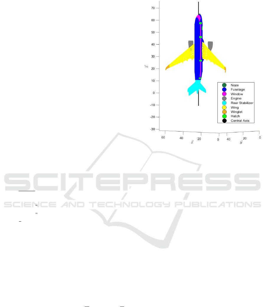
Table 1. A central axis ⃗z has also been deﬁned, so

as to convert the points from Cartesian coordinates to

cylindrical coordinates (cf. Figure 2).

The 3D point-cloud is deﬁned in Cartesian frame

cart

= {P

cart

} for i ∈



0 N



where N is the num-

ber of points of the point-cloud. A semantic label l

associated to each point of the cloud. We deﬁne the

cloud P

cyl

from P

cart

through the cylindrical coordi-

nate transformation:

∀P

cart



x y z



, P

cyl



ρ θ z



where:

ρ =

+ y

θ =











arctan(

) if x > 0

arctan(

) + sign(y) · π if x < 0

· sign(y) if x = 0 and y ̸= 0

indeterminate else

An intermediate grid in cylindrical coordinates is de-

ﬁned with steps δθ and δz. It is used to deﬁne the two

following mappings for each cell:

• R (θ, z), which contains a radius ρ as a function of

θ and z (see Figure 3a)

• L(θ,z), which describes the corresponding label l

as a function of θ and z (see Figure 3b )

For a given cell of coordinates





and

size



δθ δz



we consider the set of points

= {P

∈ P

cyl

} such that θ ∈ θ

δθ

and z ∈ z

δz

An index i

is then computed as follows

= arg max

∈P

(ρ

)

R (θ, z) = ρ

L(θ,z) = l

If the set P

contains several points with identical ρ,

the tie is broken using a majority vote on the labels of

the set.

Figure 2: Semantic point cloud obtained after vertex inter-

polation and manual labeling from an aircraft 3D mesh.

In the aircraft point-cloud considered, points la-

beled ”Winglets”, ”Engines”, and ”Rear Stabilizer”,

that are considered as non-traversable by the robot

and which can be easily truncated from the model,

were excluded. The ”Wing” label points with a ra-

dius larger than that of the surrounding fuselage are

also excluded, not only because path planning in this

area is not addressed as justiﬁed previously, but also

because their shape is not expected to be compatible

with the surface representation based on θ and z. In-

deed, several ”Wing” labeled points could have highly

variable radius, and only the one with the largest ra-

dius would be retained in the model, which is not

representative of the actual wing surface. Moreover,

this would result in the projection of the ”Wing” label

onto fuselage areas located in the same cell, which

would exclude these areas from the inspection path

calculation. From the perspective of the fuselage in-

spection, the resulting ”Wing” points are considered

as non-traversable obstacles around which the inspec-

tion should be conducted.

The semantized coordinates of a point

(ρ θ z)

and the associated label l in the se-

mantic point cloud can be directly obtained from the

grid indices (i j)

in the unfolded discrete model

ICINCO 2023 - 20th International Conference on Informatics in Control, Automation and Robotics

436

Table 1: Semantic labels and related traversability.

Label

Label Name Color

traversable?

Nose dark green 0

Fuselage blue 1

Window magenta 1

Engine grey 0

Rear Stabilizer cyan 0

Wing yellow 0

Winglet orange 0

Hatch green 0

(a)

(b)

(c)

Figure 3: 3a : Airplane Surfacic Model R (θ,z), 3b : Air-

plane Semantic Unfolded Model L(θ,z) , 3c : 3D Semantic

Point Cloud reconstructed by inverse transformation (1).

through the inverse transformation:











θ = i · δθ

z = j ·δz

ρ = R (θ,z)

l = L(θ, z)

(1)

In the model studied, the z-axis origin has been

repositioned such that the points labeled as ”Rear Sta-

bilizer” are excluded from the 2D grid. This inverse

transformation makes it possible to reconstruct a 3D

point cloud from the two surface models, as illus-

trated in Figure 3c. This will allow us then to obtain

the waypoints in the 3D space from the set of q cells

in the 2D grid. Three 2D grid layers of dimension

max

× j

max

can now be deﬁned, as follows.

Deﬁnition 3.4 ( Label Grid G ). The label at coordi-

nates (i, j) of the semantic grid G is valued as:

G(i, j) = L(i · δθ, j · δz) (2)

Deﬁnition 3.5 ( Traversability Grid B ). B is a binary

grid where

B(i, j) =

(

1 if G(i, j) is traversable

0 otherwise

(3)

Then, to avoid collisions between the inspection robot

and obstacles, a dilation is applied to B so that the

cells with a non-traversable label are dilated by a

circular structuring element with radius equal to ∆ j,

which is the length of the sensor ﬁeld projected onto

the grid.

Deﬁnition 3.6 ( Obstacle Grid O ). O is an obsta-

cle grid of dimensions i

max

× j

max

obtained by us-

ing the Connected-Component Labeling algorithm

(Chang et al., 2004) on the grid B. As a result, neigh-

bor cells q ∈ O corresponding to obstacles are as-

signed the same index, and cells corresponding to free

space are assigned 0.

3.3 Inspection Segments

From the two-dimensional grid model of the aircraft,

a full-coverage path should be determined to provide

successive inspection points fulﬁlling the required ob-

jectives and constraints. The climbing robot must per-

form a full coverage of the surface while avoiding ob-

stacles such as hatches and wings. The robot’s sen-

sor ﬁeld of view should also be aligned with the sur-

face to carry out its mission. This results in the need

for the inspection paths to be wrapped around the air-

craft’s longitudinal axis, each of them remaining in a

plane deﬁned by a constant z coordinate. In a 2D grid,

this corresponds to scanning the cells in a direction

collinear with

⃗

i. The deﬁnition of the inspection seg-

ments is performed thanks to the binary grid B. They

are sampled along the i axis between labels consid-

ered as obstacles, and they are spaced from each other

along the j axis by a distance of ∆ j = ﬂoor



sensor

2 · δz



where l

sensor

is the width scanned by the sensor on the

surface. This ∆ j parameter could be chosen smaller

than this value in order to pre-compensate for path

tracking errors by the robot. Each cell q of a segment

(corresponding to coordinates (i, j)) is stored in a vec-

tor p

, which corresponds to a path identiﬁed by index

Curved Surface Inspection by a Climbing Robot: Path Planning Approach for Aircraft Applications

437

Figure 4: Deﬁnition of the inspection segments p

visual-

ized on the G(i, j) grid (simpliﬁed version without dilata-

tion of the obstacles). The robot is represented in grey, and

the ﬁeld of its inspection sensor is shown in white. The di-

rection of the robot’s movement is represented by a black

arrow.

k (see Figure 4), and the collection of these segments

is stored in a set of inspection segments S.

Deﬁnition 3.7 ( Inspection Segment p

). A segment

of index k ∈ N

∗

, and of ﬁrst cell q

and last cell q

with respective coordinates (i

, j

) and (i

, j

), veri-

ﬁes:

• ∀q

∈ p

, j

= j

:= j

• if i

> 1, then B(i

− 1, j

) = 0

• if i

< i

max

, then B(i

+ 1, j

) = 0

The collection of these segments is initially stored

in a set of inspection segments S.

3.4 Obstacle-Based Area Decomposition

in 2D Discrete Space

The grid G is partitioned into ordered areas a

with

respect to obstacles from the grid O. This will be used

to connect the inspection segments contained in these

areas.

Deﬁnition 3.8 ( Area a

). The m-th area a

is a set

of traversable cells located between groups of non-

traversable cells with the same obstacle index, respec-

tively denoted by n

on the left border and n

on the

right border. The areas are primarily ordered along

ascending i indices, and then along the j indices. If

there exists an area a

, i < m that has the same n

and n

indices as a

, then a third index cpt is used

to distinguish them. This deﬁnes the unique identiﬁer

vector α

= [n

cpt] of the area a

. The ordered

set A stores all the identiﬁers α

The obstacle indices n

and n

take their values

from the grid O, and if there is no obstacle (i.e. a

traversable cell is located at the minimum or max-

imum i index on a given j-th line) then the default

assigned index is −1.

Remark. The variable cpt ∈ N is a counter to distin-

guish areas that are located between the same obsta-

cles of index n

and n

but are not connected along

the j-axis.

All the segments p

that belong to an area a

are

traversed in ascending order of j to determine the or-

dered set of cells Q

. It should be noted that this as-

sumes that the very starting cell of the global path will

be in position (i = 1, j = 1). Let q

and q

be the start-

ing and ending cells of p

. To determine the area a

to which a path p

belongs, we query the labeled ob-

stacle grid O to ﬁnd the obstacle identiﬁers n

and

respectively neighbors of q

and q

. Indeed, we

keep track of the last j-coordinate of the last added

path to each area a

, and this data is stored in a vec-

tor last j area at the index m. Let q

last

be the last

cell q of the last segment p

added in Q

. If q

last

is closer in the grid to q

than q

, the next segment

= {q

,..., q

} is reversed. This operation con-

sists of reordering p

in descending order of indices

n, resulting in a segment p

= {q

N−1

,..., q

}. This

procedure iterates until all the segments p

∈ S have

been inserted into Q . As a result, on average, one

inspection segment over two is reversed to sweep the

surface in a Boustrophedon pattern.

Algorithm 1 describes the corresponding pseudo-

code, and an illustration of the clustering is given in

Figure 5. The remaining step of the method is to con-

nect the inspection segments together to form the ﬁnal

global path Q .

3.5 Path Connection Between

Inspection Segments that Minimize

Gravity Constraints

The robot’s conﬁguration implies that it experiences

the least amount of effort when its vertical axis is par-

allel to gravity, that is to say when it adheres to a hori-

zontal surface. Indeed, the robot tends to slip the most

when it adheres to a vertical surface, which requires it

to deliver more power to adhere more strongly to the

wall and thus increase the frictional force that keeps it

in place. It will therefore expend less energy adhering

to the surface at the top ( θ =

) and bottom of the air-

craft ( θ = −

). Moreover, intermediate cells need to

be inserted outside of the inspection segments so that

ICINCO 2023 - 20th International Conference on Informatics in Control, Automation and Robotics

438

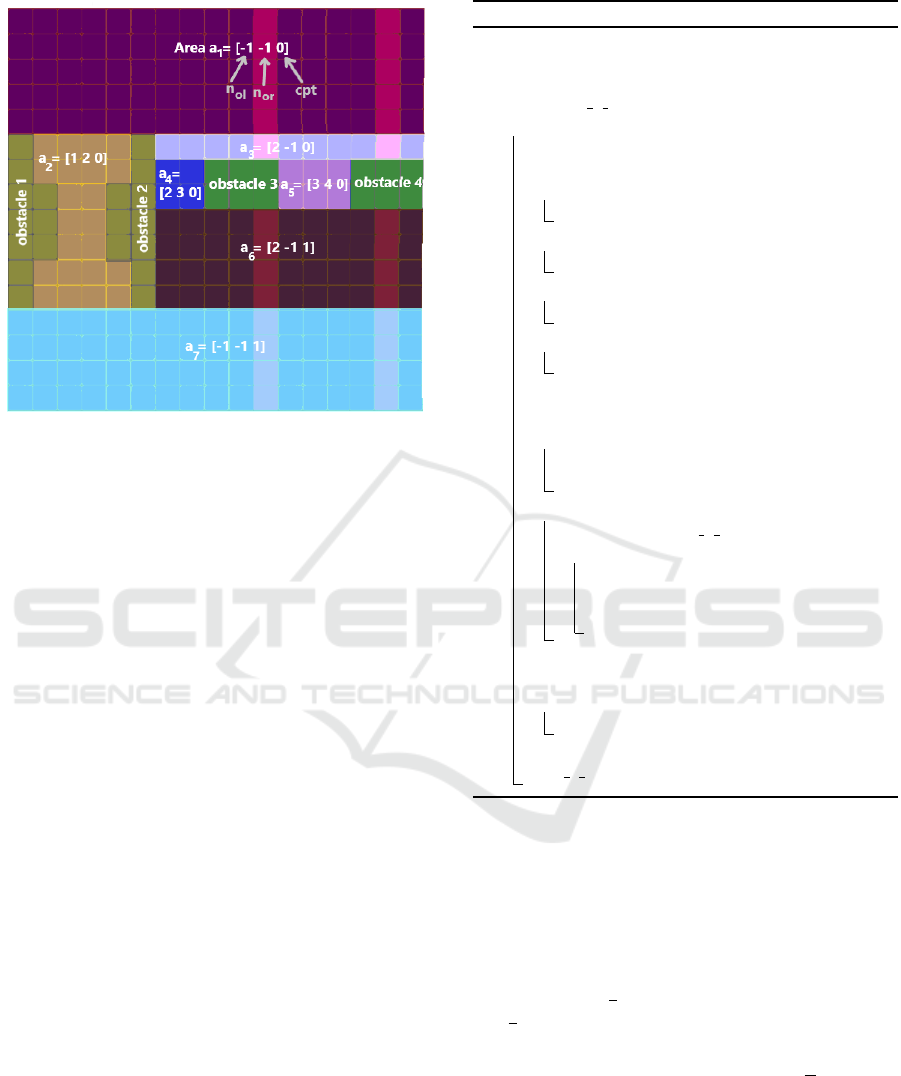
Figure 5: Example of areas numbering based on their se-

mantics and surrounding obstacles. When there are no ob-

stacles to the left of an area, n

defaults to −1 (and vice

versa for n

). In this example, we can observe that a

and

are differentiated by their value of cpt since the connec-

tion criterion is not satisﬁed, same for a

and a

the robot can move from an inspected area to an unin-

spected one, and it can also move from one segment to

another within the same area. It is preferable for the

robot to pass through the locations where the grav-

itational force is energetically less constraining. For

this purpose, a weighted version of the A

∗

algorithm is

used to plan the connecting segment (deﬁned below)

linking the last cell of the previous inspected segment

last

and the ﬁrst cell q

of a not-yet-inspected seg-

ment.

Deﬁnition 3.9 ( Connecting Segment d

). A Con-

necting Segment d

of indices k

∈ N

∗

is a seg-

ment that connects two inspection segments p

and

. Let q

and q

be the ﬁrst and last cell of d

and q

be the ﬁrst and last cell of p

. Then

veriﬁes q

= q

and q

= q

The computation process evaluates the cost f as-

sociated to the starting cell and other neighboring

cells successively until reaching the q

cell (the neigh-

borhood is deﬁned as 8-connectivity). These costs be-

tween a currently evaluated node q

cur

and one of its

neighbors q

nei

are deﬁned as:

g(q

nei

,L) = g(q

cur

,L) + c(q

nei

,L) · ∥ξ

nei

− ξ

cur

∥

(4)

f (q

nei

,L) = g(q

nei

,L) + ∥ξ

− ξ

cur

∥

(5)

where ξ

cur

, ξ

nei

, ξ

are the discrete indices (i, j) as-

sociated with cells q

cur

, q

nei

, q

, respectively. The

Algorithm 1: Ordering of the inspection segments.

Input: set S, grid O

Output: set Q

1 sets A ← {}, Q ← {[]}

2 Vector last j area ← []

3 for p

in S do

4 Integer cpt ← 0

5 cells q

← p

.begin(), q

← p

.end()

6 if q

.i > 1 then

7 n

← O(q

.i − 1,q

. j)

8 else

9 n

← −1

10 if q

.i < i

max

then

11 n

← O(q

.i + 1,q

. j)

12 else

13 n

← −1

14 Vector α ←



cpt



15 Integer m ← A. f ind(α)

16 if m is empty then

17 A.pushBack(α)

18 m ← A. f ind(α)

19 else

20 while |q

. j − last j area[m]| ̸= ∆ j and

m not empty do

21 cpt ← cpt + 1

22 α ←



cpt



23 m ← A. f ind(α)

24 q

last

= Q {m}.end().end()

25 if distance(q

last

) < distance(q

last

)

then

26 p

.reverse();

27 Q {m}.pushBack(p

)

28 last j area[m] ← q

. j

weighting function is deﬁned as :

w(q

nei

,L) =

(

1 + |cos(θ)| if L(θ, z) is traversable

∞ otherwise

(6)

where (θ, z) are the non-discretized coordinates asso-

ciated to q

nei

. θ is deﬁned such that θ ∈ [−π; π] and

such that θ = −

at the bottom of the aircraft, and

θ =

at the top. This cost factor gives more weight to

the distance between a node q

cur

and its neighbor q

nei

if it has an angular position θ far from ±

. It would

also be possible to introduce a cost function that pri-

oritizes a path crossing through certain labels over

others, for example, in cases where avoiding passage

over windows is preferable, without being an absolute

requirement. This is a way to generate a semantic-

aware path from the available graph information, as

previously proposed in (Achat et al., 2022).

Curved Surface Inspection by a Climbing Robot: Path Planning Approach for Aircraft Applications

439

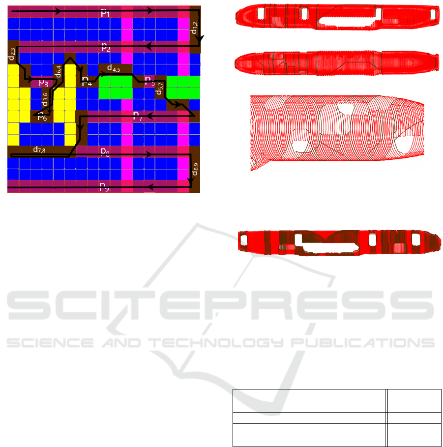
Figure 6: Final global path Q (black) vizualized in the 2D

unfolded discrete space (simpliﬁed version). It is composed

of inspection segments p

(red) and connecting segments

(brown). In this example, Q = {Q

,. . . , Q

}, with

= {p

1,2

, p

2,3

},Q

= {p

3,6

, p

6,4

},Q

{},Q

= {p

4,5

},Q

= {p

5,7

},Q

= {p

7,8

},Q

8,9

, p

All the inspection segments previously ordered by

areas are traversed in this order to be connected to-

gether in Q . Thus, the Global Path Q contains the

subsets Q

ranked in ascending order of m such as

∀Q

∈ Q and ∀p

∈ Q

, if p

belongs to a

. The

are ranked in Q

in ascending order of k. Every

subsets Q

∈ Q contains also connecting segments

between every p

such as ∀d

∈ Q

: ∃!p

∈

= q

, with q

the ﬁrst cell of d

and q

the last cell of p

. d

is inserted at the index fol-

lowing p

in Q

In the end, a comprehensive global path which in-

cludes all the inspection segments is obtained, with

additional connecting paths (see Figure 6). The spac-

ing between these segments is at most equal to half of

the sensor’s ﬁeld of view (by construction of the 2D

grid), ensuring that the entire space to be inspected

is covered. The inverse transformation (1) enables to

project back the global inspection path in the initial

3D space as illustrated in Figure 7.

4 NUMERICAL EXPERIMENTS

4.1 Path Planning Unitary Tests

This section aims to evaluate the previously presented

path planning method, speciﬁcally focusing on the

effectiveness of sorting inspection paths into areas

(a) Side view

(b) Top view

Figure 7: Global planned path with full coverage. Inspec-

tion segments are represented in red, and connecting seg-

ments that limit gravity constraints in brown.

Figure 8: Computed inspection path in the case ”Without

sorting by areas”. In this case, the length of connecting

paths (represented in brown) is signiﬁcantly increased in

comparison to the path illustrated in Figure 7.

prior to the connection process. The developed algo-

rithms have been implemented in C++ and run within

a Ubuntu 20.04 WSL Environment on a computer

equipped with Intel Core i5-10400H CPU and 16GB

RAM. Calculation times are detailed in Table 2.

Table 2: Calculation times.

Sampling of inspection segments

(ms)

0.54

Algorithm 1 (ms) 0.61

Calculation and insertion of

connecting segments (ms)

The following Table 3 presents the numerical pa-

rameters associated to the 2D grid generated from the

aircraft 3D mesh. Table 4 presents the characteris-

tics of the inspection segments that have been deﬁned

in the 2D grid. It should be noted that in our case,

the length of the sensor’s ﬁeld of view is such that its

half-length in the 2D grid ∆ j is equal to 1. This im-

plies that the robot must pass through all the grid cells

q associated with traversable labels.

A comparison was conducted between the com-

puted inspection paths in the two following cases:

• ”With sorting by area”: the global path is com-

puted with the proposed path planning method.

• ”Without sorting by area”: the global path is com-

ICINCO 2023 - 20th International Conference on Informatics in Control, Automation and Robotics

440

Table 3: Numerical characteristics of the test grid.

Longitudinal resolution δz (metres) 0.24

Angular resolution δθ (degrees) 3.6

Grid dimensions i

max

× j

max

101 × 226

Number of areas 33

puted by connecting the inspection segments to-

gether, still avoiding obstacles, but without prior

area sorting (Section 3.4).

In both cases, the length of the computed path, as well

as the number of connected waypoints were recorded

(see Table 5). It turns out that sorting the inspection

segments by the areas deﬁned between obstacles al-

lows us to halve the total distance traveled, and de-

crease by 93% the number of interpolated waypoints

to connect these segments.

Table 4: Numerical characteristics of the inspection seg-

ments generated from the test grid.

Number of inspection segments

sampled

300

Inspection segments cumulative

length in pixels (in metres)

19282

(3639 m)

Average spacing between two

consecutive waypoints (metres)

0.19

Half-length of the sensor’s range

∆ j in cells



sensor

in metres



1 cell

(0.4 m)

Table 5: Comparison of interpolated paths with and without

sorting inspection paths into areas.

Method

Without

sorting by

areas

With

sorting by

areas

Number of interpolated

waypoints

19234 1343

Path length

(in metres)

8206 4034

4.2 ROS Simulation

For illustration purposes and to eventually close the

gap with real-world deployment, a ROS simulation

has been set up to test the path-following behaviour

by a climbing robot on the surface of an aircraft. A

wheel-based robot equipped with an adhesion system

similar to the Vortex Climbing Robot (Andrikopou-

los et al., 2019) is simulated using the ROS/Gazebo

environment (see Figure 10)

. The adhesive force of

the robot is emulated by applying forces on the robot

in the opposite direction of the local surface normal.

Video: https://tinyurl.com/OneraClimbingRobotPlan

ning

Figure 9: 3D ﬁeld of surface normal vectors to the airplane

obtained through the inverse transformation of the grid N .

Figure 10: Climbing wheeled robot tracking the generated

inspection path on the surface of an aircraft, simulated in a

ROS/Gazebo environment.

For this purpose, a model of the surface normal vec-

tors of the airplane N (i, j) has been established from

a meshed model, in a similar manner to the models

R (i, j) and L(i, j). Note that N is a grid of dimen-

sions i

max

× j

max

× 3. A representation of the surface

normal vectors of the airplane is depicted in Figure 9.

In order to perform path tracking control,

the 3D position and orientation of the robot

quat)

are associated with a 2D posi-

tion and orientation in the plane deﬁned by (θ, z). The

orientation of the robot in this plane corresponds to

the projected yaw angle ψ, and its position is deﬁned

by θ and z. The odometry data provides the position

of the robot in the 3D space, namely x

, y

and z

, as

well as its orientation quat parametrized as a quater-

nion. Thus, the robot’s state in the 2D plane is de-

scribed by the coordinates (θ z ψ)

This robot local planar state is determined as fol-

lows. Firstly, the unit vector ⃗v corresponding to the

robot’s orientation in the 3D space is computed using

the quat value. Let P

1,cart

be the origin of the vector⃗v

(thus P

1,cart

is located at the center of the robot in the

3D space) and let P

2,cart

be the point located at its end-

point. These two points can be rewritten in cylindrical

coordinates similarly to Section 3.2, which gives P

1,cyl

and P

2,cyl

. The coordinates of these points in the local

2D plane are P

= (ρ

,θ

) and P

= (ρ

,θ

which allows us to determine the state of the robot as:













atan2(z

− z

,ρ

· θ

− ρ

· θ

)





(7)

Due to the discontinuity at θ = ±π, the calcu-

lated value of the angle ψ can be incorrect when the

points P

1,cyl

and P

2,cyl

are located on different sides

of this boundary. To address this issue, the value of

is adjusted within the range [−2π; +2π] based on

Curved Surface Inspection by a Climbing Robot: Path Planning Approach for Aircraft Applications

441

∈ [−π; +π]. The cells q = (i, j) of the precom-

puted ofﬂine global inspection path Q are converted

into waypoints with coordinates







i · δθ j · δz R (i · δθ, j · δz)



The path tracking performed by the robot is a

waypoint-based navigation method based on a uni-

cycle model. Thus, the robot aligns itself towards

the next waypoint by adjusting its yaw angle in the

2D plane with the angular set-point ψ

= atan2(z

−

z,ρ

· θ

− ρ

θ) using a proportional angular con-

troller. A velocity controller is then applied once the

angular error is below a small threshold. This control

logic leads to the expected correction in the 3D space

and the simulated robot model was successfully able

to track the inspection path on the surface of the air-

craft (Figure 10).

5 CONCLUSIONS AND

PERSPECTIVES

A method for planning a covering path on a curved

surface in the context of an automated inspection mis-

sion has been proposed in this paper. A 2D un-

folded model of this surface was established using

a parametrization of an input 3D model in cylindri-

cal coordinates. It was discretized to obtain two sur-

face functions, one describing the shape of the sur-

face and the other its semantics. Inspection segments

were sampled in this 2D space, taking into account

various constraints related to the robot. A method for

decomposing this discrete space into areas has been

deﬁned to order these segments efﬁciently. Connec-

tion segments have been inserted between the inspec-

tion segments and calculated to pass through locations

that minimize the robot’s efforts using a weighted A∗

search procedure. This method has been tested nu-

merically on a representative aircraft 3D mesh where

the relevance of sorting the inspection path segments

by areas was demonstrated, and in a Gazebo simula-

tion with a simpliﬁed climbing robot model.

In the context of aircraft inspection, approximating

its surface with a cylindrical parametrization presents

some limitations, e.g. to exclude the wings in the

model. It would be interesting to investigate in fu-

ture work the extension of the path planning method

to surfaces of different shapes, or the possibility of di-

viding a 3D model into multiple sub-models that can

be individually approximated by a collection of geo-

metrical primitives.

ACKNOWLEDGMENTS

This research was partially supported by DGAC

France Relance project EXAM, in the frame of the

NextGenerationEU program.

REFERENCES

Acar, E. U., Choset, H., Rizzi, A. A., Atkar, P. N., and

Hull, D. (2002). Morse decompositions for cover-

age tasks. The International Journal of Robotics Re-

search, 21(4):331–344.

Achat, S., Marzat, J., and Moras, J. (2022). Path planning

incorporating semantic information for autonomous

robot navigation. In 19th International Conference

on Informatics in Control, Automation and Robotics

(ICINCO), Lisbonne, Portugal.

Andrikopoulos, G., Papadimitriou, A., Brusell, A., and

Nikolakopoulos, G. (2019). On model-based adhesion

control of a vortex climbing robot. In IEEE/RSJ In-

ternational Conference on Intelligent Robots and Sys-

tems (IROS), pages 1460–1465.

ahnemann, R., Lawrance, N., Chung, J. J., Pantic, M.,

Siegwart, R., and Nieto, J. (2021). Revisiting boustro-

phedon coverage path planning as a generalized trav-

eling salesman problem. In 12th International Confer-

ence on Field and Service Robotics, pages 277–290.

Bugaj, M., Nov

ak, A., Stelmach, A., and Lusiak, T. (2020).

Unmanned aerial vehicles and their use for aircraft

inspection. In 2020 New Trends in Civil Aviation

(NTCA), pages 45–50.

Chang, F., Chen, C.-J., and Lu, C.-J. (2004). A linear-time

component-labeling algorithm using contour tracing

technique. Computer Vision and Image Understand-

ing, 93:206–220.

Chen, H., Fuhlbrigge, T., and Li, X. (2008). Automated

industrial robot path planning for spray painting pro-

cess: A review. In IEEE International Conference on

Automation Science and Engineering, pages 522–527.

Choset, H. and Pignon, P. (1998). Coverage path planning:

The boustrophedon cellular decomposition. In Field

and service robotics, pages 203–209.

Dahiya, C. and Sangwan, S. (2018). Literature review on

travelling salesman problem. International Journal of

Research, 5:1152–1155.

Fernandez, R. F., Keller, K., and Robins, J. (2016). Design

of a system for aircraft fuselage inspection. In IEEE

Systems and Information Engineering Design Sympo-

sium, pages 283–288.

Gabriely, Y. and Rimon, E. (2001). Spanning-tree based

coverage of continuous areas by a mobile robot. An-

nals of mathematics and artiﬁcial intelligence, 31:77–

98.

ICINCO 2023 - 20th International Conference on Informatics in Control, Automation and Robotics

442

Galceran, E. and Carreras, M. (2013). A survey on coverage

path planning for robotics. Robotics and Autonomous

Systems, 61:1258–1276.

Hasan, K. M., Reza, K. J., et al. (2014). Path planning al-

gorithm development for autonomous vacuum cleaner

robots. In International Conference on Informatics,

Electronics & Vision (ICIEV).

Liu, Y., Zhao, W., Liu, H., Wang, Y., and Yue, X.

(2022). Coverage path planning for robotic quality

inspection with control on measurement uncertainty.

IEEE/ASME Transactions on Mechatronics, 27:3482–

3493.

Mineo, C., Pierce, S., Nicholson, I., and Cooper, I.

(2017). Introducing a novel mesh following technique

for approximation-free robotic tool path trajectories.

Journal of Computational Design and Engineering,

4:192–202.

Qin, L., Jin, Z., Suo, S., Zhang, C., Qiao, K., and Liu, J.

(2022). Design and research of a wall climbing robot

with ducted fan for aircraft appearance inspection. In

International Conference on Sensing, Measurement &

Data Analytics in the era of Artiﬁcial Intelligence (IC-

SMD).

Rai, K., Madan, L., and Anand, K. (2014). Research paper

on travelling salesman problem and its solution using

genetic algorithm. International Journal of Innovative

Research in Technology, 1(11):103–114.

orme, J. and Edwards, T. (2018). A comparison of path

planning algorithms for robotic vacuum cleaners. In

BSc report, KTH Royal Institute of Technology.

Starbuck, B., Fornasier, A., Weiss, S., and Pradalier, C.

(2021). Consistent state estimation on manifolds for

autonomous metal structure inspection. In IEEE In-

ternational Conference on Robotics and Automation

(ICRA), pages 10250–10256.

Wang, C., Gu, J., and Li, Z. (2019). Switching motion con-

trol of the climbing robot for aircraft skin inspection.

In IEEE International Conference on Fuzzy Systems.

Wu, H. and Tang, Q. (2023). Robotic spray painting path

planning for complex surface: boundary ﬁtting ap-

proach. Robotica, 41(6):1794–1811.

Wu, Q., Lu, J., Zou, W., and Xu, D. (2015). Path plan-

ning for surface inspection on a robot-based scanning

system. In IEEE international conference on mecha-

tronics and automation (ICMA), pages 2284–2289.

Zelinsky, A., Jarvis, R. A., Byrne, J. C., and Yuta, S. (1993).

Planning paths of complete coverage of an unstruc-

tured environment by a mobile robot. In Proceedings

of International Conference on Advanced Robotics,

volume 13, pages 533–538.

Curved Surface Inspection by a Climbing Robot: Path Planning Approach for Aircraft Applications

443