Comparative Evaluation of Metaheuristic Algorithms for
Hyperparameter Selection in Short-Term Weather Forecasting
Anuvab Sen
1
a
, Arul Rhik Mazumder
2 b
, Dibyarup Dutta
3 c
, Udayon Sen
4 d
,
Pathikrit Syam
1
e
and Sandipan Dhar
5 f
1
Electronics and Telecommunication, Indian Institute of Engineering Science and Technology, Shibpur, Howrah, India
2
School of Computer Science, Carnegie Mellon University, Pittsburgh, Pennsylvania, U.S.A.
3
Information Technology, Indian Institute of Engineering Science and Technology, Shibpur, Howrah, India
4
Computer Science and Technology, Indian Institute of Engineering Science and Technology, Shibpur, Howrah, India
5
Computer Science and Engineering, National Institute of Technology, Durgapur, West Bengal, India
Keywords:
Genetic Algorithm, Differential Evolution, Particle Swarm Optimization, Meta-Heuristics, Artificial Neural
Network, Long Short Memory Networks, Gated Recurrent Unit, Auto-Regressive Integrated Moving Average.
Abstract:
Weather forecasting plays a vital role in numerous sectors, but accurately capturing the complex dynamics
of weather systems remains a challenge for traditional statistical models. Apart from Auto Regressive time
forecasting models like ARIMA, deep learning techniques (Vanilla ANNs, LSTM and GRU networks) have
shown promise in improving forecasting accuracy by capturing temporal dependencies. This paper explores
the application of metaheuristic algorithms, namely Genetic Algorithm (GA), Differential Evolution (DE), and
Particle Swarm Optimization (PSO) to automate the search for optimal hyperparameters in these model archi-
tectures. Metaheuristic algorithms excel in global optimization, offering robustness, versatility, and scalability
in handling non-linear problems. We present a comparative analysis of different model architectures integrated
with metaheuristic optimization, evaluating their performance in weather forecasting based on metrics such
as Mean Squared Error (MSE) and Mean Absolute Percentage Error (MAPE). The results demonstrate the
potential of metaheuristic algorithms in enhancing weather forecasting accuracy & helps in determining the
optimal set of hyper-parameters for each model. The paper underscores the importance of harnessing advanced
optimization techniques to select the most suitable metaheuristic algorithm for the given weather forecasting
task.
1 INTRODUCTION
Weather forecasting is the use of science and technol-
ogy to predict future weather conditions in a specific
geographical area. It plays a vital role in agriculture,
transportation, and disaster management. Traditional
methods rely on physical models, but they may strug-
gle to capture the complex dynamics of weather sys-
tems accurately. To address this, deep learning tech-
niques have emerged, leveraging large datasets to im-
a
https://orcid.org/0009-0001-8688-8287
b
https://orcid.org/0000-0002-2395-4400
c
https://orcid.org/0009-0008-9012-2816
d
https://orcid.org/0009-0006-6575-6759
e
https://orcid.org/0009-0003-2370-182X
f
https://orcid.org/0000-0002-3606-6664
prove forecasting accuracy by uncovering hidden pat-
terns.
Recently, time series models like recurrent neu-
ral networks (RNNs) have become popular in weather
forecasting due to their ability to capture temporal
dependencies. However, the standard RNN model
often faces challenges like exploding and vanishing
gradient problems, making it difficult to capture long-
term dependencies. To address this, Long Short-Term
Memory (LSTM) models have emerged as superior
alternatives (Hochreiter and Schmidhuber, 1997), ex-
celling at capturing sequential information from long-
term dependencies. Additionally, Gated Recurrent
Unit (GRU) networks (Jing et al., 2019), another class
of RNNs, have shown promise in sequence predic-
tion problems. GRUs mitigate the vanishing gradient
problem by employing update and reset gates, signif-
238
Sen, A., Mazumder, A., Dutta, D., Sen, U., Syam, P. and Dhar, S.
Comparative Evaluation of Metaheuristic Algorithms for Hyperparameter Selection in Short-Term Weather Forecasting.
DOI: 10.5220/0012187300003595
In Proceedings of the 15th International Joint Conference on Computational Intelligence (IJCCI 2023), pages 238-245
ISBN: 978-989-758-674-3; ISSN: 2184-3236
Copyright © 2023 by SCITEPRESS – Science and Technology Publications, Lda. Under CC license (CC BY-NC-ND 4.0)

icantly improving the modeling of long-term depen-
dencies. Moreover, due to their reduced parameter
count, GRUs generally require less training time than
LSTMs.
Achieving optimal performance with GRUs of-
ten requires manual tuning of hyperparameters such
as learning rate, batch size, and number of epochs,
which is time-consuming and labor-intensive. To
overcome this, the paper proposes the use of meta-
heuristic algorithms like Genetic Algorithm (GA),
Differential Evolution (DE), and Particle Swarm Op-
timization (PSO) to automate the search for the best
hyperparameter settings, ultimately enhancing fore-
casting accuracy. These metaheuristic algorithms of-
fer advantages in tackling challenges related to train-
ing and optimizing complex neural network architec-
tures.
Weather forecasting saw a notable improvement
with the introduction of metaheuristic algorithms to
optimize deep learning models like GRU. Leverag-
ing the global optimization capabilities of these al-
gorithms, weather forecasting models achieved bet-
ter performance by efficiently exploring and exploit-
ing the search space to find optimal solutions. This
is essential for accurately predicting complex and
dynamic weather systems. Moreover, metaheuristic
algorithms exhibit robustness, versatility, and scala-
bility, enabling them to handle non-linear and non-
convex problems effectively. Integrating them with
existing models facilitates adaptation to evolving
challenges in weather prediction.
Genetic Algorithm (GA) (Man et al., 1996), based
on the Darwinian theory of Natural Selection, was
developed in the 1960s but gained popularity in the
late 20th Century. It falls under the broader class of
Evolutionary Algorithms and is widely used to solve
search problems through bio-inspired processes like
mutation, recombination, and selection. Differential
Evolution (DE) (Storn and Price, 1997) is another
population-based metaheuristic algorithm that itera-
tively improves a population of candidate solutions
to optimize a problem. Particle Swarm Optimiza-
tion (PSO) (Kennedy and Eberhart, 1995), inspired
by bird flocking or fish schooling behavior, maintains
a swarm of particles that move in the search space to
find the optimal solution.
This paper presents a comparative analysis of
architectures for weather forecasting using a meta-
heuristic optimization algorithm. We evaluate these
architectures based on metrics like Mean Squared
Error (MSE) and Mean Absolute Percentage Error
(MAPE). Additionally, we curate a comprehensive
weather dataset spanning 10 years to train our best
forecasting model. Leveraging the Gated Recurrent
Unit (GRU) architecture with Differential Evolution
optimization, we achieve superior accuracy and per-
formance in predicting weather conditions.
2 RELATED WORK
Hyperparameter optimization is a critical research
area for achieving high-performance models. Tech-
niques like Random Search (Radzi et al., 2021), Grid
Search (Shekar and Dagnew, 2019), Bayesian Opti-
mization (Masum et al., 2021), and Gradient-based
Optimization (Maclaurin et al., 2015) are used to find
optimal hyperparameter configurations. Each method
offers trade-offs in computational efficiency, explo-
ration of search space, and exploitation of solutions.
Genetic Algorithms were first utilized for modi-
fying Artificial Neural Network architectures in 1993
(B¨ack and Schwefel, 1993), inspiring various nature-
based algorithms’ applications to deep-learning mod-
els (Katoch et al., 2020). While many works com-
pare evolutionary algorithms on computational mod-
els, no previous study comprehensively compares the
three most promising evolutionary algorithms: Ge-
netic Algorithm, Differential Evolution, and Particle
Swarm Optimization, across multiple computational
architectures. These algorithms stand out due to
their iterative population-based approaches, stochas-
tic and global search implementation, and versatility
in optimizing various problems. Moreover, no re-
search has explored these metaheuristics across such
a diverse range of models. Although many papers
analyze metaheuristic hyperparameter tuning on Ar-
tificial Neural Networks (Orive et al., 2014), (Ne-
matzadeh et al., 2022) and Long Short-Term Mem-
ory Models (Wang et al., 2022), they are few meta-
heuristic hyperparameter tuning methods for Auto-
Regressive Integrated Moving Average and Gated Re-
current Networks. Additionally, a thorough inves-
tigation of papers on metaheuristic applications for
ARIMA and GRU tuning reveals that none of them
utilize the three evolutionary algorithms (GA, DE,
PSO) discussed in this study.
3 BACKGROUND
3.1 Metaheuristics
3.1.1 Genetic Algorithm
Genetic Algorithm (GA) is a metaheuristic algorithm
based on the evolutionary process of natural selection,
the key driver of biological evolution mentioned in
Comparative Evaluation of Metaheuristic Algorithms for Hyperparameter Selection in Short-Term Weather Forecasting
239

Darwin’s theory of evolution. Similar to how evolu-
tion generates successful individuals in a population,
GA generates optimal solutions to constrained and
unconstrained optimization problems. The summa-
rized pseudocode of the Genetic Algorithm is shown
in Algorithm 1.
Algorithm 1: Genetic Algorithm.
Input : Population Size N ∈ (5, 10),
Chromosome Length L, Termination
Criterion
Output: Best Individual
1 Initialize the population with N random
individuals;
2 while Termination Criterion is not met do
3 Evaluate fitness f (x
i
) for all individual x
i
in population;
4 Select parents p
1
, p
2
from the population
for mating. Use a Roulette Wheel
Selection scheme.;
5 Create a new population by applying
uniform crossover: and mutation
operations on the selected parents to get
c
i
;
6 Replace the current population with the
new population;
7 end
8 return best individual in the final population;
Genetic Algorithm initializes a population, selects
parents for mating using a custom fitness function,
and produces new candidate solutions by applying
mutations and crossover to previous solutions. We
utilized a Roulette Wheel Selection scheme and a
Uniform Crossover scheme and ran Genetic Algo-
rithm for 10 generations.
3.1.2 Differential Evolution
Differential Evolution (DE) is a population-based
metaheuristic used to solve non-differentiable and
non-linear optimizations. DE obtains an optimal so-
lution by maintaining a population of candidate so-
lutions and iteratively improving these solutions by
applying genetic operators.
Similar to the Genetic Algorithm, Differential
Evolution begins by randomly initializing a pop-
ulation and then generating new solutions using
crossover and mutation operators, shown below. It
uses a custom fitness function when deciding to re-
place previous solutions.
A pseudocode implementation for Differential
Evolution is provided in Algorithm 2. We cycled
through the selection, mutation, and crossover opera-
tions of Differential Evolution for 10 generations be-
Algorithm 2: Differential Evolution.
Input : Population Size N ∈ (5, 10),
Dimension D, Scale Factor F,
Crossover Probability CR,
Termination Criterion
Output: Best individual
1 Initialize the population with N random
individuals in the search space;
2 while Termination Criterion is not met do
3 for each individual x
i
in the population
do
4 Select three distinct individuals x
r
1
,
x
r
2
, and x
r
3
from the population;
5 Generate a trial vector v
i
by mutating
x
r
1
, x
r
2
, and x
r
3
using the differential
weight F;
v
i
= x
r
1
+ F × (x
r
2
− x
r
3
) (1)
6 Perform crossover between x
i
and v
i
to produce a trial individual u
i
with
the crossover probability CR;
u
j,i
=

v
j,i
, if p
rand
(0, 1) ≤ CR
x
j,i
else

(2)
7 if the fitness of u
i
is better than the
fitness of x
i
then
8 Replace x
i
with u
i
in the
population;
9 end
10 end
11 end
12 return the best individual in the final
population;
fore terminating the number of runs.
3.1.3 Particle Swarm Optimisation
Particle Swarm Optimization (PSO) is a population-
based metaheuristic algorithm inspired by the social
behavior of bird flocking or fish schooling. It aims
to find optimal solutions by simulating the move-
ment and interaction of particles in a multidimen-
sional search space. Like other metaheuristic algo-
rithms, PSO begins with the initialization of particles
and arbitrarily sets their position and velocity. Each
particle represents a potential solution, and their po-
sitions and velocities are updated iteratively based on
a fitness function and the global best solution found
by the swarm. The summarized pseudocode of PSO
is displayed in Algorithm 3.
ECTA 2023 - 15th International Conference on Evolutionary Computation Theory and Applications
240

Algorithm 3: Particle Swarm Optimization.
Input : Number of particles N ∈ (5, 10),
Max Iterations M, Termination
Criterion
Output: Global Best Fitness
1 Initialize the particle’s position with a
uniformly distributed random vector:
x
i
∼ U(b
lo
, b
up
);
2 Initialize the particle’s velocity:
v
i
∼ U(−|b
up
− b
lo
|, |b
up
− b
lo
|);
3 Calculate Global Best Fitness f(g);
4 for i = 1 to M do
5 for j = 1 to N do
6 Update the particle’s position:
x
i
← x
i
+ v
i
;
7 Update the particle’s velocity: v
i
←
ωv
i
+ c
1
r
1
(p
i
− x
i
) + c
2
r
2
(p
g
− x
i
);
8 Evaluate fitness f(p
i
);
9 if f(p
i
) < f(g) then
10 f(g) = f(p
i
)
11 x
n
= x
n+1
12 end
13 end
14 end
In Algorithm 3, b
lo
& b
up
are bounds on the range of
values within which the initialization parameters will
be initialized.
3.2 Models
3.2.1 Auto-Regressive Integrated Moving
Average
The Auto-Regressive Integrated Moving Average
(ARIMA) (Harvey, 1990) is a time series forecasting
model that extends the autoregressive moving average
(ARMA) model (Brockwell and Davis, 1996). Their
advantage, is that they can reduce a non-stationary se-
ries into a stationary series and thus provide a broader
scope of forecasting capabilities. An ARIMA model
is composed of three components:
1. Auto-regression (AR) measures a variable’s de-
pendence on its past values, enabling predictions
of future values. In ARIMA, the p hyperparam-
eter represents this order and the number of past
values used for current observations. A time se-
ries {x
i
} is said to be autoregressive of order p if:
x
i
= Σ
p
j=1
α
j
x
i− j
+ w
i
(3)
where w
i
is the white noise and α
i
are non-zero
constant real coefficients.
2. Integration (I) assimilates time series data, trans-
forming non-stationary series into stationary ones
through differencing current and previous values.
The hyperparameter d denotes the magnitude of
differencing needed for data stationarity.
3. Moving Average (MA) accounts for past error
residuals’ impact on the variable value. Like the
AR component, it predicts current values using
past error combinations. The q hyperparameter
determines the number of lagged error terms for
the prediction. A time series has a moving aver-
age of order q if:
x
i
= w
i
+ β
1
w
i−1
+ .... + β
q
w
i−q
(4)
where {w
i
} is the set of white noise and β
i
are
non-zero constant real coefficients.
3.2.2 Artificial Neural Network
Artificial Neural Network (ANN) is a computational
model inspired by the human brain’s neural circuits.
A core part of Deep Learning, ANNs detect patterns,
learn from historical data, and make informed deci-
sions.
Neural networks consist of artificial neurons ar-
ranged in a multilayer graph. There are three types
of layers: input, hidden, and output. Input data is
processed through at least one hidden layer, and each
neuron in the hidden layer learns patterns from inputs
x
i
(size n) and produces output h using Equation 5.
h = ρ(b
j
+
n
∑
i=1
w
i
x
i
) (5)
In the equation above b
j
and w
i
represent the bi-
ases and weights from each input node respectively.
The function ρ is the activation function designed to
introduce nonlinearity and bound output values.
Training the neural network follows supervised
learning, where biases b
j
and weights w
i
are adjusted
to achieve the optimal output. During training, an er-
ror function f compares the ANN’s output with the
desired output for each data point in the training set.
The errors are then corrected through Backpropaga-
tion (Kelley, 1960), a stochastic gradient descent al-
gorithm. The initial weights are adjusted according to
Equations 6 and 7 below:
w := w− ε
1
∂f
∂w
(6)
b := b− ε
2
∂f
∂b
(7)
Comparative Evaluation of Metaheuristic Algorithms for Hyperparameter Selection in Short-Term Weather Forecasting
241

3.2.3 Long Short-Term Memory
Long Short-Term Memory (LSTM) is a type of Re-
current Neural Network (RNN) that maintains short-
term memory over time by preserving activation pat-
terns. Unlike standard feed-forward neural networks,
LSTM’s feedback connections allow it to handle data
sequences, making it ideal for time series analysis
(Hochreiter and Schmidhuber, 1997).
LSTM utilizes specialized memory cells that re-
tain activation patterns across iterations. Each LSTM
memory cell comprises four components: a cell, an
input gate, a forget gate, and an output gate. The cell
serves as the memory for the network. It retains es-
sential information throughout the processing of the
sequence. The Input Gate updates the cell. This pro-
cess is done by passing the previously hidden layer
(h
t−1
) information (weights w
i
and biases b
i
) and cur-
rent state x
t
into a sigmoid function σ as outlined in
the Equation 8.
i = σ(w
i
[h
t−1
, x
t
] + b
i
) (8)
The Forget Gate is responsible for deciding which in-
formation is thrown away or retained. This function
is very similar to the Input Gate and outlined in Equa-
tion 9 below.
f = σ(w
f
[h
t−1
, x
t
] + b
f
) (9)
The Output Gate is responsible for determining the
next hidden state and is important for predictions. The
output function follows from the same functions de-
scribed with the Input Gate and Forget Gate.
o = σ(w
o
[h
t−1
, x
t
] + b
o
) (10)
3.2.4 Gated Recurrent Unit Networks
The Gated Recurrent Unit (GRU) is an RNN architec-
ture that overcomes some limitations of LSTM while
delivering comparable performance. GRUs excel at
capturing long-term dependencies in sequential data.
GRUs are computationally less expensiveand eas-
ier to train than LSTMs due to their simpler architec-
ture. They merge the cell and hidden state, removing
the need for a separate memory unit. GRUs also use
gating mechanisms to control information flow within
the network. The GRU relies on a series of gates sim-
ilar to the LSTM. The Update gate determines how
much of the previous hidden state to keep and how
much of the new input to incorporate. It is computed
as:
z
t
= σ(W
z
· [h
t−1
, x
t
]) (11)
where W
z
is the weight matrix associated with the up-
date gate, h
t
− 1 is the previous-hidden state, x
t
is the
input at time step t and σ is the sigmoid activation
function. The Reset Gate determines how much of
the previous hidden state to forget. It is computed as:
r
t
= σ(W
r
· [h
t−1
, x
t
]) (12)
where W
r
is the weight matrix associated with the re-
set gate. The smaller the value of the reset gate r
t
is,
the more the state information is ignored. The Current
Memory Content is calculated as a combination of the
previous hidden state and the new input, controlled by
the update gate:
˜
h
t
= tanh(W · [r
t
⊙ h
t−1
, x
t
]) (13)
where W is the weight matrix and ⊙ denotes element-
wise multiplication. The Hidden State at time step t is
updated by considering the current memory content.
h
t
= (1− z
t
) ⊙ h
t−1
+ z
t
⊙
˜
h
t
(14)
where ⊙ denotes element-wise multiplication.
4 DATASET DESCRIPTION
We have created a dataset
1
by scraping from the offi-
cial website of Government of Canada (Canada and
Change, 2023), by taking weather related data for
the region of Ottawa from date 1
st
January 2010 to
31
st
December 2020. It has the following features:
date, time (in 24 hours), temperature (in
◦
Celsius),
dew point temperature (in
◦
Celsius), relative humid-
ity (in %), wind speed (in kilometers/hours), visibil-
ity (in kilometers), pressure (in kilopascals) and pre-
cipitation amounts (in millimeters). It also had a few
derived features like humidity index and wind chill,
which we did not take into account to keep our list of
features as independent as possible from each other.
The compiled data set comprised 96,408 rows of data
for 8 variables, where each row represents an hour.
5 PROPOSED APPROACH
This section describes the implementation of meta-
heuristic algorithms from Section 2 for time series
forecasting using various models. Each model is
trained on a training set to find optimal hyperpa-
rameters, evaluated by mean average percentage er-
ror (MAPE) on the test data.In preprocessing, miss-
ing data was handled. The precipitation amount col-
umn had significant missing data and was dropped.
The temperature column had a small amount of miss-
ing data (0.03% of total data). Models forecasted
24 hours into the future based on every 3 hours of
1
Dataset link: https://doi.org/10.7910/DVN/PJISJU
ECTA 2023 - 15th International Conference on Evolutionary Computation Theory and Applications
242

data. The StandardScaler function from sklearn.pre-
processing library (Pedregosa et al., 2011) was used
for standardization. The dataset was split into train
dataset (D
train
), validation dataset (D
val
), and test
dataset (D
test
). Train data was from Jan 1, 2010, to
Dec 31, 2015; validation data from Jan 1, 2016, to
Dec 31, 2016; and test data from Jan 1, 2017, to Dec
31, 2020.
5.1 Auto-Regressive Integrated Moving
Average
We employed the ARIMA (p, d, q) model from
statsmodels.tsa.arima.model, utilizing temperature as
the sole feature due to its univariate nature. Mean
squared error (MSE) served as the fitness function
for metaheuristic algorithms such as GA, DE, & PSO.
The hyperparameter search space for each algorithm
was limited to (0, 5) for p, (0, 3) for d, and (0, 5) for
q, considering our machine’s limitations. Differential
Evolution yielded the best MAPE of 2.31.
5.2 Artificial Neural Networks, Long
Short Term Memory, Gated
Recurrent Networks
To ensure consistency among the deep learning mod-
els, we maintained a 3-layer architecture with varying
neuron counts for input, GRU/LSTM layers, and out-
put. GRU and LSTM models used 8 features from
the previous three timesteps (3 hours) as input, with
36, 64, and 24 neurons for input, GRU/LSTM layers,
and output, respectively. The ANN model had 24 in-
put features, with 64, 36, and 24 neurons for input,
hidden layer, and output, respectively.
Table 1: Best set of hyperparameters (in the order learning
rate, batch size, and epochs, respectively) for ANN, LSTM,
and GRU averaged over 5 runs.
Metaheuristics Hyperparameters ANN LSTM GRU
GA
Learning Rate 0.0001 0.0001 0.0001
Batch Size 80 80 80
Epochs 527 860 758
DE
Learning Rate 0.0005 0.75 0.075
Batch Size 200 24 20
Epochs 8 1000 200
PSO
Learning Rate 0.1061 0.2964 0.4176
Batch Size 41 66 202
Epochs 84 33 61
For the ANN model, the dataset shapes were:
x
train
: (52558, 24), y
train
: (52558, 24), x
val
: (8760,
24), y
val
: (8760, 24), x
test
: (35016, 24), and y
test
:
(35016, 24). For GRU and LSTM models, the dataset
shapes considered time steps: x
train
: (53558, 3, 8)
and similar shapes for other splits. All networks uti-
lized the ReLU activation function & employed im-
plemented metaheuristic algorithms to optimize batch
size, epochs, and learning rates using Mean Squared
Error as the loss metric. The best hyperparameter sets
for each model are summarized in Table 1. MAPE
plots were generated for each set of hyperparameters.
6 RESULTS AND DISCUSSION
We implemented the proposed metaheuristics-based
optimal hyperparameters’ selection, evaluating three
deep learning models (ANN, GRU, LSTM) for algo-
rithm suitability while maintaining consistent three-
layer architecture. All values shown were averaged
over five trials, and all figures displayed used stan-
dardized units. Additionally, we explored other mod-
els, including the machine learning model ARIMA.
The paper’s code can be found below.
2
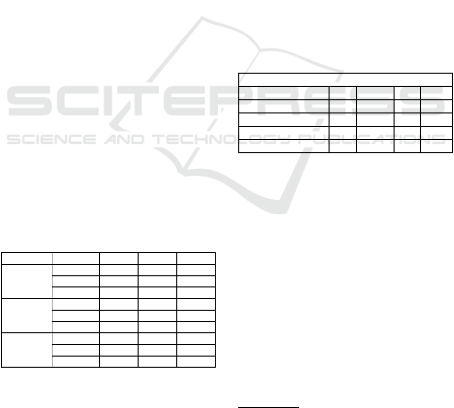
Table 2: MAPE comparison of different meta-heuristics for
ANN, ARIMA, GRU, and LSTM averaged over 5 runs.
MAPE - Mean Absolute Percentage Error
Meta-heuristics ANN ARIMA GRU LSTM
Differential Evolution 1.15 2.31 1.75 1.65
Particle Swarm (PSO) 1.95 2.85 1.86 1.98
Genetic Algorithm (GA) 1.97 3.28 1.93 1.97
Manual Selection 2.09 4.34 1.98 1.99
We utilized Standard Scaler for improved conver-
gence and stability during model training with sea-
sonal data. Scaling prevents dominant features and
enhances the models’ learning effectiveness. Data
preprocessing, including scaling and handling sea-
sonal patterns, is crucial for boosting forecasting
model performance. The deep learning model’s in-
put and output layers have different neuron counts
based on requirements. GRU and LSTM use eight
features from previous time steps, including the cur-
rent one, leading to 36, 64, and 24 neurons in the in-
put, neural network, and output layers, respectively.
For the ANN model, features from three-hour time
steps are concatenated, resulting in an input feature
size of 24. Consequently, the input layer has 64 neu-
rons, while the hidden and output layers contain 36
and 24 neurons, respectively. Mean Squared Error
(MSE) is employed to minimize training loss. The ex-
periments show that the ANN model optimized with
Differential Evolution (DE) outperforms other mod-
els with different optimization algorithms. DE with
2
Code link: https://github.com/pathikritsyam/ECTA
Comparative Evaluation of Metaheuristic Algorithms for Hyperparameter Selection in Short-Term Weather Forecasting
243

Figure 1: Predicted plots for temperature for the next 24 hours starting from the N-th hour for the best ANN DE Model.
ANN achieves the lowest Mean Absolute Percentage
Error (MAPE) of 1.15, followed by DE with LSTM.
DE consistently outperforms GA and PSO in terms
of MAPE for each model, and performs superiorly
across all models compared to GA and PSO. DE is
Figure 2: 24-hour ahead forecast plot for the best perform-
ing model.
chosen as the effective metaheuristic algorithm due to
its efficient search space exploration and adaptability
across generations. Its capability to handle continu-
ous parameter spaces makes it well-suited for opti-
mizing neural network hyperparameters. Neverthe-
less, the optimal optimization algorithm choice may
vary depending on the dataset and task. The meta-
heuristic algorithms consistently outperform manual
hyperparameter search. Additionally, deep learning
models (ANN, GRU, LSTM) outperform ARIMA in
forecasting accuracy. ARIMA’s limitation is its in-
ability to capture complex non-linear patterns in data,
resulting in inferior performance. The results clearly
show that Differential Evolution (DE) outperforms
both Particle Swarm Optimization (PSO) and Genetic
Algorithm (GA) in terms of Mean Absolute Percent-
age Error (MAPE) across different models used in the
study. DE’s superior performance can be attributed
to several key factors. It effectively explores the
search space and exploits promising regions for opti-
mal solutions. The mutation operator introduces ran-
dom perturbations to prevent early convergence. The
crossover operator facilitates the exchange of promis-
ing features, speeding up the convergence process.
The selection operator preserves the fittest individu-
als, enhancing the quality of solutions. PSO demon-
strates good performance but falls slightly behind
DE. It suffers from premature convergence, limiting
its ability to reach the global optimum, which could
be an explanation for its performance. GA, on the
other hand, shows relatively poor performance com-
pared to both DE and PSO. It could possibly be due
to slow convergence, and the fixed encoding scheme
may limit its ability to effectively search through the
vast hyperparameter space if the solution requires a
specific combination of hyperparameters. The find-
ings indicate that deep learning models (ANN, GRU,
LSTM) outperform the ARIMA model in forecasting
accuracy.
Metaheuristic algorithms (DE, GA, PSO) con-
sistently outperform manual hyperparameter search.
Among the three, DE proves to be the most effective
ECTA 2023 - 15th International Conference on Evolutionary Computation Theory and Applications
244

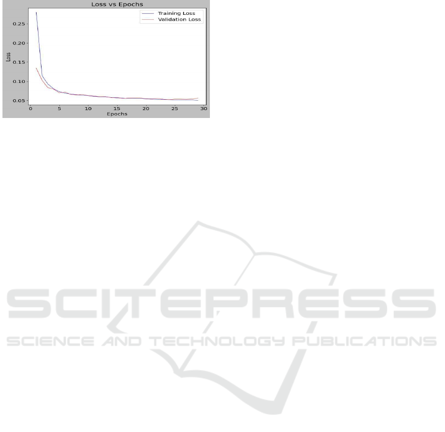
Figure 3: Training & Validation loss plots vs Epochs for the
Best ANN DE Model.
algorithm, outperforming both GA and PSO.
7 CONCLUSION
This paper applies metaheuristic algorithms to opti-
mize hyperparameters in deep learning models like
Artificial Neural Networks, GRUs, LSTMs, and
ARIMA for better performance. We find that Dif-
ferential Evolution (DE) outperforms Genetic Algo-
rithm (GA) and Particle Swarm Optimization (PSO)
in short-term weather forecasting. DE’s ability to ex-
plore and exploit the search space effectively leads to
optimal solutions. While PSO performs well, it can
sufferfrom prematureconvergence,and GA may have
slow convergence and limitations for hyperparameter
configurations. In the future, this approach can be ex-
tended to explore other evolutionary-based feature se-
lections for various time series applications.
REFERENCES
Brockwell, P. J. and Davis, R. A. (1996). Arma mod-
els. Introduction to Time Series and Forecasting, page
81–108.
B¨ack, T. and Schwefel, H.-P. (1993). An overview of evo-
lutionary algorithms for parameter optimization. Evo-
lutionary Computation, 1(1):1–23.
Canada, E. and Change, C. (2023). Government of canada
/ gouvernement du canada.
Harvey, A. C. (1990). Arima models. Time Series and
Statistics, page 22–24.
Hochreiter, S. and Schmidhuber, J. (1997). Long short-term
memory. Neural Computation, 9(8):1735–1780.
Jing, L., Gulcehre, C., Peurifoy, J., Shen, Y., Tegmark, M.,
Soljacic, M., and Bengio, Y. (2019). Gated orthogonal
recurrent units: On learning to forget. Neural Compu-
tation, 31(4):765–783.
Katoch, S., Chauhan, S. S., and Kumar, V. (2020). A review
on genetic algorithm: Past, present, and future. Multi-
media Tools and Applications, 80(5):8091–8126.
Kelley, H. J. (1960). Gradient theory of optimal flight paths.
ARS Journal, 30(10):947–954.
Kennedy, J. and Eberhart, R. (1995). Particle swarm op-
timization. Proceedings of ICNN’95 - International
Conference on Neural Networks, 4:1942–1948.
Maclaurin, D., Duvenaud, D., and Adams, R. P. (2015).
Gradient-based hyperparameter optimization through
reversible learning.
Man, K., Tang, K., and Kwong, S. (1996). Genetic algo-
rithms: Concepts and applications [in engineering de-
sign]. IEEE Transactions on Industrial Electronics,
43(5):519–534.
Masum, M., Shahriar, H., Haddad, H., Faruk, M. J., Valero,
M., Khan, M. A., Rahman, M. A., Adnan, M. I., Cuz-
zocrea, A., and Wu, F. (2021). Bayesian hyperpa-
rameter optimization for deep neural network-based
network intrusion detection. 2021 IEEE International
Conference on Big Data (Big Data).
Nematzadeh, S., Kiani, F., Torkamanian-Afshar, M., and
Aydin, N.(2022). Tuning hyperparameters of machine
learning algorithms and deep neural networks using
metaheuristics: A bioinformatics study on biomedi-
cal and biological cases. Computational Biology and
Chemistry, 97:107619.
Orive, D., Sorrosal, G., Borges, C., Martin, C., and Alonso-
Vicario, A. (2014). Evolutionary algorithms for
hyperparameter tuning on neural networks models.
26th European Modeling and Simulation Symposium,
EMSS 2014, pages 402–409.
Pedregosa, F., Varoquaux, G., Gramfort, A., Michel, V.,
Thirion, B., Grisel, O., Blondel, M., Prettenhofer,
P., Weiss, R., Dubourg, V., et al. (2011). Scikit-
learn: Machine learning in python. Journal of ma-
chine learning research, 12(Oct):2825–2830.
Radzi, S. F., Karim, M. K., Saripan, M. I., Rahman, M. A.,
Isa, I. N., and Ibahim, M. J. (2021). Hyperparam-
eter tuning and pipeline optimization via grid search
method and tree-based automl in breast cancer predic-
tion. Journal of Personalized Medicine, 11(10):978.
Shekar, B. H. and Dagnew, G. (2019). Grid search-based
hyperparameter tuning and classification of microar-
ray cancer data. In 2019 Second International Con-
ference on Advanced Computational and Communi-
cation Paradigms (ICACCP), pages 1–8.
Storn, R. and Price, K. (1997). Differential evolution – a
simple and efficient heuristic for global optimization
over continuous spaces - journal of global optimiza-
tion.
Wang, S., Ma, C., Xu, Y., Wang, J., and Wu, W. (2022).
A hyperparameter optimization algorithm for the lstm
temperature prediction model in data center. Scientific
Programming, 2022:1–13.
Comparative Evaluation of Metaheuristic Algorithms for Hyperparameter Selection in Short-Term Weather Forecasting
245