Maritime Dynamic Resource Allocation and Risk Minimization Using

Visual Analytics and Elitist Multi-Objective Optimization

Mayamin Hamid Raha, Md. Abu Sayed, Monica Nicolescu, Mircea Nicolescu and Sushil Louis

Department of Computer Science and Engineering, University of Nevada, 1664 N. Virginia Street, Reno, NV 89557, U.S.A.

Keywords:

Resource Allocation, Intensity Maximization, Visualization, Risk Minimization, Threat Evaluation, Multi-

Objective Optimization, Fitness Function.

Abstract:

Enhancing the safety of protected regions around Navy vessels is one of the most challenging research topics

in maritime domains. Robust tactical resource allocation depends on understanding of how the placement,

conﬁgurations, orientations of multiple assets affect both the area and intensity of coverage around the ships.

Towards this end, we built a unique resource allocation problem where we apply a randomized genetic algo-

rithm for searching through a space of 2

144

possible parameters representing area coverage, orientation of 6

tactical assets. Our elitist genetic algorithm yielded a maximum ﬁtness value of 90%, 98%, 100% within 50,

150 and 300 generations respectively. Moreover, we put forward a distinctive constrained dynamic resource

allocation problem speciﬁc to USS Arleigh Burke Destroyer model (DDG-51), where the assets are defenses

and coastal guards having binoculars. To solve this, we have used a cross-generational elitist selection based

evolutionary algorithm (EA) where our objective is to maximize area of coverage and minimize risk simulta-

neously. It is a non-deterministic polynomial-time hard (NP-Hard) problem which required searching through

a space of 2

parameters and resulted in a ﬁtness value of 98% within 35 generations. Furthermore, we

present two novel visualization techniques addressing both types of resource allocations.

1 INTRODUCTION

In maritime domains, dealing with the wide range

of possible threats to large ships requires a strategic

placement of sensory and defensive resources (Be-

naskeur et al., 2007) . Large number of maritime

surveillance tasks are focused towards effectively op-

erating ﬁxed and mobile surveillance assets which is

also known as resource allocation (RA) (Dridi et al.,

2012) . With dynamically evolving data about the

presence of hostile ships, there is a ever increasing

demand of intelligent systems to support in proactive

decision making through multi-level resource alloca-

tion (Mishra et al., 2015) . Radar, sonar, infrared, and

visual are some of the many sensors that are com-

monly present in Navy ships. Some of these assets

come with spherical area of coverage, whereas, some

assets have a conical area of coverage deﬁned as a

ﬁeld of view (FOV). In case of tactical assets, the se-

curity level around a ship depends on both the area

of coverage of the assets (how far it can cover) and

the efﬁciency or strength of coverage at various loca-

tions (intensity of coverage). While some assets have

almost the same coverage efﬁciency at any range or

angle from a principal axis (for conical ﬁeld of view),

others have varying efﬁciency that decays with linear

or angular distance from the principal axis. Identify-

ing hostile vessels ahead of time (Carlson et al., 2019)

can help ships plan their trajectory accordingly and

allocate assets such that the level and range of protec-

tion around the vessel is increased. Moreover, visu-

alizing target area around ships can help to conduct

better surveillance by aiding prompt decision making

(Davis et al., 2016) . For searching through a space

of large number of solutions, evolutionary algorithms

have proven to be one of the best optimization tech-

niques where model performance is explainable and

not a black box (Grefenstette, 1993). Elitist evolu-

tionary algorithms are often preferred due to their ten-

dency of converging faster by retaining copies of best

individuals through radical recombination (Eshelman,

1991) .

Motivated by the potentials of area based intensity

maximization in maritime security enhancement and

the lack of similar research in this ﬁeld, we propose

the following:

• A generalized resource allocation (GRA) prob-

lem for multiple assets based on area of coverage

Raha, M., Sayed, M., Nicolescu, M., Nicolescu, M. and Louis, S.

Maritime Dynamic Resource Allocation and Risk Minimization Using Visual Analytics and Elitist Multi-Objective Optimization.

DOI: 10.5220/0012190100003543

In Proceedings of the 20th International Conference on Informatics in Control, Automation and Robotics (ICINCO 2023) - Volume 1, pages 54-63

ISBN: 978-989-758-670-5; ISSN: 2184-2809

where the linear range of coverage, angular cover-

age range and orientations are all dynamic. These

are the parameters that are selected by our EA for

optimization. We deﬁned 6 locations to place the

resources, any asset can be placed in any six loca-

tions provided that it maximizes area of coverage

and that location is not already occupied by an-

other asset. The set of resources and their speciﬁ-

cations are ﬂexible and can be changed according

to any hypothetical or real ship model.

• A visualization technique using Pygame, for area

based generalized resource allocation. Assets are

represented with triangular shapes representing

their area of coverage, and they can be placed in 6

different locations on the ship.

• A constrained dynamic resource allocation (DRA)

problem for a DDG-51 ship model where the as-

sets are 2 set of defenses with 2 different ﬁxed

locations and 4 different possible orientations per

defense. Furthermore, the asset sets include 6

coastal guards having binoculars, who can be

placed in 16 different locations on the ship and

can have 8 different values for orientation place-

ment.

• A technique for risk proﬁle (intensity) and area

based coverage visualization for multiple assets of

DDG-51 Navy ship using OpenCV (Figure 2).

Our work focuses on ﬁnding optimum set of as-

set allocation parameters using elitist genetic algo-

rithm and providing corresponding 2D visualization

for navy ships.

2 RELATED WORK

With growing complexity of maritime threats, allo-

cation of navy resources (sensors/defenses) is of key

interest and has many relevant applications. Some

include RA for maritime search and rescue (SAR)

(Ai et al., 2019), (Guo et al., 2019), emergency

people evacuation (Zhang et al., 2017), power al-

location of multi-satellites for maritime mobile 6G

communication (Hassan et al., 2023), straddle car-

rier scheduling in maritime container terminal at im-

port (Dkhil et al., 2018), beam scheduling problem

for multifunctional radar (Jeong et al., 2023), threat

evaluation and weapon allocation (TEWA) (Par-

adis et al., 2005), weapon-target assignment (WTA)

(Zhang et al., 2023), risk assessment (Malik et al.,

2014) and many more (Cao et al., 2022; Dridi et al.,

2012; Qian et al., 2022; Hattaway, 2008).

Recently, a rapid growth of visual analytics tools

has taken place (Stasko et al., 2007; Willems et al.,

Figure 1: An example of generalized RA using visualiza-

tion interface of Pygame where A-F are locations for asset

placement.

2009) . Mostly, such tools offer graph visualization

(Cleveland and McGill, 1988) and coordinate plots

(Inselberg, 2009). Although these allow us to derive

better understanding of the data and aid decision mak-

ing process, it is only very recent that researchers have

started incorporating output from visualization tech-

niques in risk assessment (Malik et al., 2014).

Integration of visual analytics in maritime domain

can provide deeper insights into many problems such

as risk assessment, threat evaluation, intent recogni-

tion (Carlson et al., 2019) and resource allocation. Al-

though we see the use of visual data in various RA

problems targeted towards SAR applications (Malik

et al., 2014), there are rarely any available systems

for visualization of tactical resources (mainly sensors

and defenses) . Visualization of the level of protection

provided by various sensors and defenses following

any allocation pattern can lead to better threat eval-

uation and enhanced understanding of point and area

defense. Having data related to location of various red

ships near a blue ship can only be of little signiﬁcance

in real time scenarios, where prompt decision making

is crucial. Algorithmic approach towards modeling

RA for tactical resources of navy ships can yield bet-

ter outcome due to maximum utilization of limited re-

sources and enhanced security. RA along with avail-

able visualization technique can lead to better antici-

pation of risk and threat level associated with complex

maritime scenarios. With this idea, we have deﬁned

and solved two different RA problems for navy ships

utilizing evolutionary algorithms and visual analytics.

Maritime Dynamic Resource Allocation and Risk Minimization Using Visual Analytics and Elitist Multi-Objective Optimization

+ 45

𝑜

- 45

𝑜

principal axis, defense

𝒍

𝟏

𝒍

𝟐

𝒍

𝟑

𝒍

𝟒

𝒍

𝟓

𝒍

𝟖

+ 65

𝑜

𝒍

𝟔

principal axis, coast guard with binocular

- 65

𝑜

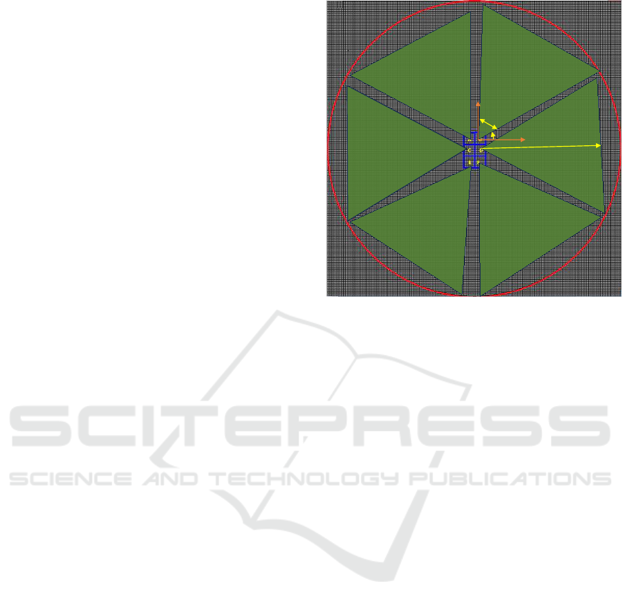
Less protected region (in red)

representing lower intensity of coverage

Highly protected region (in green)

representing higher intensity of coverage

𝒍

𝟕

Figure 2: Tactical Asset Intensity Visualization for Risk

Minimization using OpenCV.

h3 h4 h5

𝛼

(a)

𝑂

𝑙

(b)

Figure 3: Structure of chromosome for generalized Re-

source Allocation and Multi-objective Resource Allocation

speciﬁc to DDG-51 shown in (a) and (b) respectively.

3 METHODOLOGY

In this section, we will discuss our algorithm frame-

work and its speciﬁcation for GRA and MOEA for

DDG-51.

3.1 CHC Selection Based Genetic

Algorithm

Genetic algorithms (GA) differ from other search al-

gorithms due to their ability to overcome local max-

ima by starting search from a random set of solutions

(Goldberg, 1987). Instead of providing one single

solution, GAs provide a set of solutions to a given

problem (Louis and Zhao, 1995). Each of these so-

lutions contain the search parameters and these so-

lutions are called chromosomes (also known as indi-

vidual). A set of chromosomes is known as a pop-

ulation. Different sets of chromosomes create dif-

ferent set of populations over different generations.

GAs select superior individuals from parent popula-

tion through a selection procedure and retain supe-

rior individuals while introducing diversity through

crossover and mutation processes. GAs can be of

various type depending on the method of selection,

crossover and mutation. Cross-generational elitist se-

lection (CHC) is a non traditional GA (Whitley and

Sutton, 2012), which combines parent and child pop-

ulation and keeps half of the chromosomes with best

ﬁtness values. This strategy retains the best individu-

als from one generation to another. In this way, CHC

based GAs can ﬁnd solutions of very complex search

space within a few generations.

3.2 Generalized Area Coverage Based

Resource Allocation and

Visualization

We have deﬁned the GRA as a set up where 6 assets

can be placed in 6 ﬁxed locations (namely A, B, C,

D, E, F) of a rectangular region representing a ship

(see Figure 1). The objective to ﬁnd which dynamic

asset conﬁguration is the best ﬁt for each of the 6

pre-deﬁned locations provided that we are placing the

assets sequentially and one location cannot be occu-

pied by more than one asset. By best ﬁt we refer to

the amount of area an asset covers based upon var-

ious parameters such as linear coverage (h), angular

coverage(θ) and orientation. Therefore, the asset type

is not ﬁxed. The assets can be anything such as de-

fense, sensors, coast guards, etc. All the assets have

a FOV ranging between +60

◦

\-60

◦

, i.e., 120

◦

is the

maximum possible angular coverage for each asset.

The linear coverage range of the assets can be from

1 km to 256 km. We chose this linear range to in-

crease the complexity of search space. By orientation

(α) in GRA problem, we refer to the angle by which

an asset can rotate anticlockwise from the x axis of its

coordinate system. At ﬁrst, we make all calculations

required for height, angle and orientation (h, θ and α)

considering the center of the Pygame interface as the

origin. Therefore, there is a single coordinate system

for all assets with the center of the Pygame window

as origin. Later, all calculations are performed on the

transformed coordinate system speciﬁc to each asset.

For instance, we can see the x and y axes for asset

placed in location B in Figure 1. In this case, the ori-

entation values range from 1

◦

to 360

◦

. Here, the loca-

tion (l) of the assets are static parameters. We use tri-

angular shapes to represent assets having sector-like

ﬁeld of view. The heights of the triangles representing

ICINCO 2023 - 20th International Conference on Informatics in Control, Automation and Robotics

the assets, namely h1-h6, indicate the linear coverage

of assets. The FOV angles and orientations are rep-

resented by parameters named (θ

- θ

) and (α

-α

)

respectively (see Figure 1). Therefore, the parame-

ter sets of (h, θ, α) values are deﬁned by the search

space. For this problem we are using a chromosome

of length 144, where there are 6 height values, 6 corre-

sponding angle values and 6 different values for orien-

tations from transformed positive x axis. Our chromo-

some structure is visualized in Figure 3a. The height,

angle and orientation values have a binary encoding,

comprising of 8, 7 and 9 bits respectively. Here, all

the parameters (h, θ, α) are dynamic, thus resulting

in a huge search space. This approach makes this GA

ﬂexible to be tuned according to any model of navy

ships with unique set of assets.

Area of Coverage Based Fitness Function. For ﬁt-

ness function calculation, we considered the percent-

age of area covered inside a circle. For this we used

the Pygame library to create a gray color display of

size 970 x 970, where 1 pixel represents 0.5 km in

real space. We drew a 512 x 512 grid to make calcu-

lations easier. Hence, there are total 940,900 pixels in

the Pygame display interface and the whole window

represents an area of 262,144 square km. Then we

drew a circle having radius of 128 grid units where

each grid unit is equivalent to 3.78 pixels. Finally, we

placed triangles (resources) from a starting location of

positive x axis in anti-clockwise direction of each of

our six coordinates in our Pygame screen which can

be seen in Figure 1. We are considering all the tri-

angles to be isosceles triangle, since in case of ships,

any asset’s ﬁeld of view is equally distributed from

principal axis of rotation. Every triangle starts from

an angle α (in Figure 3a) from the positive x axis

in anti-clockwise direction where α can have values

from 1

◦

to 360

◦

. Each isosceles triangle can have an

adjacent angle (θ) value from 1

◦

to 120

◦

and height

values (named h1-h6) ranging from 1 to 256 units (see

Figure 3a). For drawing the triangles using Pygame,

the library requires 3 coordinate points of a triangle:

2 adjacent sides of isosceles triangle have one point in

common, which give us one of the three coordinates.

We calculated the remaining coordinates of end points

of each of 3 sides of triangles by solving 3 trigono-

metric equations for each side. We considered the

trigonometric equation of a line whose perpendicu-

lar makes an angle p from the positive x axis and that

line is q angle away from positive x axis (Algorithm

1). We did this calculation to determine the orienta-

tion values and place the triangles (asset covered area)

in the Pygame visualization window using the θ and

α values which can be seen in Figure 4 and Figure

Figure 4: A sample of GRA based on solution generated

by our algorithm where height values are = [139, 178, 177,

225, 123, 217] and θ values are = [96, 115, 43, 70, 51, 2],α

values are =[235, 114, 236, 56, 346] where population size

= 50 and Generation number = 70, Area covered (inside

circle) = 75 percent.

5. In this way we do similar calculation for each tri-

angles with respect to each given location point on

a transformed coordinate system (see Algorithm 1).

The transformation is done respect to the origin of

the circle whose pixel location in the Pygame window

and our original coordinate system is (485, 485) (see

Algorithm 2). Once the coordinates of each sides end

point are found, we draw green color ﬁlled triangles

using Pygame’s gfxdraw library’s drawFilledTrigon()

function. Our algorithm is designed to deal with over-

lap of coverage of area from multiple assets using vi-

sual analytics. Since we are considering the intensity

of coverage to have the same value for each pixel irre-

spective of the number of assets that cover that area,

we used pixel-wise visual cue for calculating covered

area around ship. Once the assets are placed and vi-

sualized, our algorithm takes input from Pygame’s

visual grid and counts the number of pixels having

green color within the circular region to calculate the

effective covered area in target region (circular re-

gion). When a pixel has green color RGB value then

it is considered as covered, provided that it is within

the circumference of the circular region. This is in or-

der to compute the area that our asset placement has

covered within a certain circular boundary.

Once the coordinates of each sides end point

is found we draw green color ﬁlled triangles using

Pygame’s gfxdraw library’s drawFilledTrigon() func-

tion.

Area Covered Calculation. For area coverage cal-

culation, we calculate the number of green pixels in-

side the boundary of the circle and multiply it with

pixel size (see Equation 2). The area of circle is calcu-

Maritime Dynamic Resource Allocation and Risk Minimization Using Visual Analytics and Elitist Multi-Objective Optimization

Figure 5: height1-height6 = [221, 199, 255, 130, 31, 127]

and θ1-θ6 =[37, 84, 63, 40, 73, 28], α1-α6 =[97, 239, 220,

195, 286, 215] where population size = 100 and Generation

number = 103, Area covered (inside circle) = 82 percent.

Algorithm 1: Calculates the 3 corner coordinates of each

triangle with respect to transformed coordinate system.

Input: List of heights, FOV angles and orientation

angles(q) from positive x axis in

transformed coordinate system, p angles

(the angles made by perpendiculars of each

side of triangles with positive x axis)

Result: 3 corner coordinates of a triangle in

transformed coordinate

system(x,ycoordinatevalues);

a1 = 270 + q;

a2 = q + p/2;

a3 = 270 + q + p;

foreach p in angles (where p[i] > 0 do

xcos(a1) + ysin(a1) = 0;

xcos(a2) + ysin(a2) = height;

xcos(a3) + ysin(a3) = 0;

end

lated using Equation 1, where the radius of the circle

represents 256 km according to the maximum linear

coverage range of each assets for this problem. For

calculation of area covered inside circle by triangles,

we used the Equation 2. Here, trianglePixelCount is

the number of pixels whose RGB pixel value is green

and are inside circular boundary. Pygame window

size here is 512 x 512 pixels, therefore the pixel size

is 0.73 µm. Finally, for calculation of percentage of

area covered, we use Equation 3. We can see how our

display looks with various height, theta, alpha values

in Figure 4.

CircularArea = 3.146 ∗ (radius)

(1)

AreaCovered = pixelSize ∗ trianglePixelCount (2)

Fitness = (AreaCovered/CircularArea)∗ 100 (3)

Algorithm 2: Calculates the 3 corner coordinates of each

triangle with respect to original coordinate system.

Input: List of 3 corner coordinates of a triangle in

transformed coordinate system, i.e. list of

3 (x,y) coordinate values and coordinate of

a given pixel location on ship’s rectangular

area

Result: 3 corner coordinates of a triangle in

original coordinate system (x,y)

coordinate values;

foreach index in range len(coordinate_solutions)

coordinate_solutions[index][0] =

coordinate_solutions[index[0] +

location_point[0];

coordinate_solutions[index][1] =

coordinate_solutions[index][1] +

location_point[1];

end

Algorithm 3: Calculates the ﬁtness value for each member

of chromosome.

Input : List principal axis and locations in form of

pixel coordinates of all 8 assets,

FOV_angle

Result: combined ﬁtness value of a pixel resulting

from all the allocated assets;

asset_coverage = 0

for i = 0 to 6 do

binocular =

b_coordinate.append(b_location[i])

for i in range width do

for j in range height do

angular_distance = Calculate β from

each principal axis;

if angular_distance <= FOV_angle

then

asset_coverage + =

Intensity(eDistance, minDist,

maxDist, angular_coverage, β,

maximum_angularRange,

mapping,

intensity_distribution_pattern,

c);

else

return 0.0;

return asset_coverage;

3.3 Intensity and Area of Coverage

Based Resource Allocation

This RA approach is based on constraints imposed by

the assets of DDG-51 where we are considering allo-

cation of 2 defenses having a maximum linear cov-

erage range of 14 km and 6 coastal guards having

binoculars represented with visual sensors having a

maximum linear coverage range of 20 km. For the de-

fenses, one pixel represents 1 km and for visual sen-

ICINCO 2023 - 20th International Conference on Informatics in Control, Automation and Robotics

sors each pixel represents 1.5 km. The locations for

defenses are ﬁxed and each of them can have 4 pre-

deﬁned different orientations. The locations of the vi-

sual sensors are dynamic and 16 different locations

have been deﬁned along the borders of the ship model.

The coastal guards can be placed at any of these 16 lo-

cations and each of these mobile assets can have 8 dif-

ferent orientations. Here we have manually deﬁned 8

possible orientations values that each of these coastal

guards can have in order to reduce the complexity of

search space. The GA searches through each of these

8 different possible orientations for coastal guard as-

sets. Our chromosome has all binary values. It con-

tains 8 different orientation values where the ﬁrst two

are for defenses (2 bits each), the next 6 values are

for orientation of visual sensors (3 bits each), and the

succeeding 6 values (4 bits each) represent the loca-

tion of the visual sensors. In this case there are fewer

parameters compared to the generalized GA for area

based RA, since speciﬁc model of ships have particu-

lar range of orientations and distance coverage, which

results in reduced search space.

Multi-Objective GA Fitness Function for DDG-51.

We have taken into consideration the fact that the in-

tensity of coverage from each assets is not of equal

magnitude in every location around the ship. Inten-

sity values degrade with distance and angle from the

direction where it is pointed (also known as principal

axis). In order to model the distribution of intensity

based on linear distance, orientation and area of cov-

erage, we built a visual analytic algorithm, based on

OpenCV, and we designed a set of intensity deteriora-

tion functions to achieve this effect (see Algorithm 4).

This enables us to know the combined effect of orien-

tations and allocations of multiple static and mobile

assets at any point of time and can be used in ﬁtness

function for our GA since it can easily tell which area

is comparatively less covered by the current set of as-

set allocations (see Algorithm 3). In Algorithms 3

and 4, the variable eDistance refers to the euclidean

distance of a pixel from a principal axis (PA) of an

asset, minDist refers to the minimum coverage range

of an asset, maxDist refers to the maximum coverage

range of asset, β refers to the angular distance of a

pixel from PA of an asset, mapping refers to the scal-

ing parameter, and b_coordinate refers to the location

of coast guards with binoculars.

In our ﬁtness function, we have two main objec-

tives:

• Maximize the area covered by assets around Navy

ships and

• Maximize the strength of coverage, which implies

reduced risk in the protected zone.

The summation of pixel values having combined in-

tensity values from multiple assets help us meet both

of our objectives simultaneously, i.e., higher intensity

value of the entire image represents more area be-

ing covered along with higher strength of coverage.

Both pixel intensity values and number of pixels hav-

ing an intensity of coverage value greater than zero

contribute in overall ﬁtness value calculation of each

image generated by our visualization.

The way we achieve this effect, is by searching

through each pixel of image generated by our visu-

alization technique and assigning an intensity value

to it from every asset. We add intensity values of all

pixels in the image and assign that value and a ﬁtness

value for a particular set of allocation parameters gen-

erated by our multi-objective evolutionary algorithm

(see Algorithm 3).

In order to further optimize the calculations in ﬁt-

ness function, for every pixel of the image generated

by our visual analytic algorithm we check its angu-

lar distance from principal axis of each asset and cal-

culate ﬁtness value for it only if it falls within the

range of coverage speciﬁc to each asset (see Algo-

rithm 3). In our visual analytic helper functions we

are using inverse normalization to model the change

of intensity value with respect to distance for visual

sensors of binocular and piece-wise function for the

same in case of defenses. We refer to this as in-

tensity_distribution_pattern in Algorithm 3 and Al-

gorithm 4. Variable c is a hyper parameter with val-

ues within a range of .01 to 1. The FOV_angle vari-

able represents the maximum ﬁeld of view a speciﬁc

asset can have, for example: for coastal guards the

FOV_angle is 130

◦

(+65

◦

\-65

◦

) and for defenses the

FOV_angle is 90

◦

(+45

◦

\-45

◦

Additionally, we also have built functions to

model the intensity of coverage for other possible as-

sets such as radar, sonar sensors with spherical or cir-

cular area of coverage (see Algorithm 4). Although

we only display visualization from defenses and con-

ical FOV assets, spherical assets can also be repre-

sented using our Algorithm 4. Radar and Sonar sen-

sors differ at the rate at which their intensities decays

with linear and angular distance, due to which the in-

tensity_distribution_pattern variable is set to two dif-

ferent types, "radar_exponent" and "sonar_exponent"

respectively.

We calculate the ﬁnal intensity of coverage of a

pixel by combining the value of linear intensity (based

on euclidean distance from principal axis) and angu-

lar intensity (using Equation 4). We calculate the in-

tensity of coverage value of a pixel only when β (the

angular distance from principal axis of an asset) falls

within the maximum angular coverage region which

Maritime Dynamic Resource Allocation and Risk Minimization Using Visual Analytics and Elitist Multi-Objective Optimization

is unique to each asset. To compute β we use vector

dot product and calculate the cosine of the angle by

dividing the dot product of two vectors representing

line segments by the product of their magnitudes (see

Equation 4).

Sector_Intensity = 1 − (2 ∗ β/(max_coverage) (4)

When a pixel falls within β range, then for calcula-

tion of intensity we follow Algorithm 4: this returns

an intensity value corresponding to each pixel, which

in turn is used by Algorithm 3 to iterate through all

pixels of a visualization and calculate a ﬁtness value

for a chromosome.

Algorithm 4: Calculating the intensity of a pixel with

respect to an asset.

Input : eDistance, minDist, maxDist,

angular_coverage, β,

maximum_angularRange,

mapping,intensity_distribution_pattern,c

Result: intensity value of a pixel resulting from

one asset placed at a particular location;

if eDistance < minDist or eDistance > maxDist

then

return 0;

if intensity_distribution_pattern = "piece_wise"

then

if eDistance > 0 and eDistance < 0.025 *

maxDist then

retrun 0.9;

else if eDistance >= 0.025 * maxDist and

eDistance < 0.045 * maxDist then

return 0.7;

else if eDistance >= 0.045 * maxDist and

eDistance < 0.2 * maxDist then

retrun 0.2;

else

return 0.05;

else if intensity_distribution_pattern = "inv_norm"

then

return 1 - ((eDistance -

minDist)/(maxDist-minDist);

else if intensity_distribution_pattern =

"radar_exponent" then

return 1/e

(c∗eDistance)/(maxDist−minDist)

;

else if intensity_distribution_pattern =

"sonar_exponent" then

return 1/e

(c∗(eDistance−minDist))

;

else

return 0;

3.4 Common Parameters Used in both

Approaches

Through experimentation we found that probability

of mutation of 0.05 and probability of cross over of

0.9 works best for our generalized resource alloca-

tion and DDG-51 speciﬁc resource allocation prob-

(a)

(b)

(c)

Figure 6: Average of best, mean and worst ﬁtness curves for

RA of DDG-51 ship for 35, 70 and 150 generations in (a),

(b) and (c) respectively.

lem. For the GAs used to address both problems we

used CHC-based selection with µ value of 2, where µ

refers to the number of parents selected by the GA at

a time before crossover and mutation takes place. We

used 30 different random seeds and we averaged the

minimum, maximum and average ﬁtness of our GA

in every generation over these 30 random seeds. We

did this in order to conﬁrm that the result we obtained

was not an outcome of random initial set of chromo-

somes that the GA started working with. This can be

seen in Figures 6a, 6b and 6c.

ICINCO 2023 - 20th International Conference on Informatics in Control, Automation and Robotics

Table 1: Parameters and Maximum Fitness values (Area covered) for generalized RA having dynamic parameters.

Pop &

Gen No.

Crossover

and

Mutation

Rate

Static

parameters

Dynamic

parameters

Fitness

(%)

50 , 37 0.9, 0.05 l h,θ,α 69

50 , 70 0.9, 0.05 l h,θ,α 75

100 , 103 0.9, 0.05 l h,θ,α 82

100 , 150 0.9, 0.05 l h,θ,α 98

200 , 300 0.9, 0.05 l h,θ,α 100

300 , 450 0.9, 0.05 l h,θ,α 100

Table 2: Parameters and Maximum Fitness values multi-objective RA.

Pop &

Gen No.

Crossover

Rate

Mutation

Rate

Static

parameters

Dynamic

parameters

Fitness(%)

26, 39 0.9 0.05 h,θ α, l 97

50, 75 0.9 0.05 h,θ α, l 97

100, 150 0.9 0.05 h,θ α, l 98

4 EXPERIMENT

In this section, we evaluate the performance of our

generalized RA and DDG-51 speciﬁc constrained RA

by varying the hyper parameter values. We ran our

evolutionary algorithm for various number of gener-

ations to see if it has an impact on the results (Table

1). For all the experiments we used a hybrid computer

having Intel(R) Core(TM) i9-9900 KF processor, 32

GB RAM and NVDIA GeFORCE RTX 3060 GPU.

In Table 1, we show the population and generation

number used by our GRA algorithm, along with the

crossover-mutation rates, dynamic parameters, and

best ﬁtness value. We ran each of our GA iteration

through 30 random seeds and average the best, min-

imum and average ﬁtness value per iteration to en-

sure that GA results are not some random results in-

ﬂuenced by the initial set of chromosomes. For each

random seed we take the best ﬁtness values and av-

erage them for each generation. In the best ﬁtness

column we indicate the maximum value of those aver-

ages from generation number 0 to generation number

Parameter l refers to the locations on the ship

where asset can be placed. The dynamic parameters

h, θ, α represents the linear coverage, ﬁeld of view

angles and orientations of assets respectively. From

Table 1 it is evident that running the algorithm for

higher number of generations yields better ﬁtness val-

ues. Finally, for 300 generations with a population

size of 200, leads towards ﬁnding set of parameters

that give 100% of area coverage. We infer that ﬁnding

a set of chromosomes that yield 100% ﬁtness value

within relatively small number of generations for such

a large search space might have been possible due to

the simplicity of constraints imposed upon the param-

eters. For instance, we represented the area of cover-

age of each resource to be simply triangular (which is

not the case with real life assets), and the whole grid

size was 512 x 512 pixels only. If we took a greater

Pygame window size with more complex representa-

tion of sensor coverage then GA might have not found

a set of solution resulting in 100% area of coverage

within 300 generation only.

To explore the applicability of our approach for

real life ships with dynamic location parameters, we

also experiment with the MOEA that we built for

DDG-51 that takes into account the speciﬁc linear, an-

gular coverage ranges of its resources along with the

constraints imposed upon it. From Table 2, we see

that running our MOEA for greater number of gen-

erations with larger population size does not have a

signiﬁcant impact on our ﬁtness value. This is due to

the fact that in our second experiment we have built

an algorithm that offers an enhanced representation

of area of coverage in addition to intensity of cover-

age. Our elitist selection based GA searches through

possible combinations of orientations and locations.

Since DRA has constraints on each asset’s linear and

angular coverage ranges, these fall under the category

of static parameter. Orientation and location are dy-

namic parameters in this case.

5 RESULTS

For the generalized RA, we used population sizes

of 50 and 100 with varying numbers of generations

(Table1). From Table 1 we can see that when we let

the generalized RA run for more number of genera-

tions we obtained better results. Even for a general-

ized version of the problem with 2

144

parameters, our

Maritime Dynamic Resource Allocation and Risk Minimization Using Visual Analytics and Elitist Multi-Objective Optimization

elitist evolutionary algorithm was able to ﬁnd good re-

source allocations parameters within 150 generations

(Table1). For MOEA, upon using population size of

26, 50 and 100 for generation number 39, 75 and 150

respectively as hyper parameters for our MOEA (see

Table 2), we found that within around 25 generations

the ﬁtness values converge to 98%. These sets of solu-

tions can now be used for allocating resources on Ar-

leigh Bruke Destroyer ship for maximization of area

of coverage and risk minimization (meaning overall

higher strength of coverage). We have calculated av-

erage of best, mean and and worst ﬁtness across 30

random seeds for each generations and noticed that

the mean ﬁtness value starts from 40% ﬁtness value

and reaches a value of 80% within less than 10 gen-

erations and by 25 generations it ﬁnds the optimum

set of solutions. Maximum ﬁtness starts somewhere

around 70% and reaches 96% ﬁtness values within

less than 10 generations.

6 CONCLUSION

We formulated two novel resource allocation (RA)

problems for navy ships. The generalized version

of RA focuses on maximization of area of coverage

around ships and ﬁnds solutions having 98% area cov-

erage within a given circular boundary. The second

version of the RA problem was deﬁned considering a

DDG-51 ship’s dimensions and ranges of its available

resources. We found that our optimization approach

was able to ﬁnd solutions representing the location

and orientation of the resources ensuring 98% risk

minimization and area of coverage. Our novel visual

analytic algorithm is capable of generating visualiza-

tion of combined intensity of coverage also known

as heatmaps around DDG-51 at any point of time.

Moreover, tuning the GA for incorporating data based

on location of multiple ships in real time, can lead

to resource allocation in real time and parallel pro-

cessing can help with generating faster outputs. This

opens doors for future works related to integrating

dynamic threatmaps with our multi-objective evolu-

tionary algorithm to enhance the level of protection

around ships in multi-agent scenarios (MAS).

ACKNOWLEDGMENTS

This work has been supported by the Ofﬁce of Naval

Research award N00014-21-1-2234.

REFERENCES

Ai, B., Li, B., Gao, S., Xu, J., and Shang, H. (2019). An in-

telligent decision algorithm for the generation of mar-

itime search and rescue emergency response plans.

IEEE Access, 7:155835–155850.

Benaskeur, A., Bossé, É., and Blodgett, D. (2007). Com-

bat resource allocation planning in naval engage-

ments. Technical report, DEFENCE RESEARCH

AND DEVELOPMENT CANADA VALCARTIER

(QUEBEC).

Cao, X., Zhang, H., and Peng, M. (2022). Collaborative

multiple access and energy-efﬁcient resource alloca-

tion in distributed maritime wireless networks. China

Communications, 19(4):137–153.

Carlson, L., Navalta, D., Nicolescu, M., Nicolescu, M.,

and Woodward, G. (2019). Multinomial hmms for in-

tent recognition in maritime domains. In Proceedings

of the 18th International Conference on Autonomous

Agents and MultiAgent Systems, pages 1856–1858.

Cleveland, W. S. and McGill, M. (1988). Dynamic graphics

for statistics wadsworth & brooks. Paciﬁc Grove, CA.

Davis, A., Vincent, C., Otenti, N., and Parolin, A. (2016).

Aerial precision 3-d ground surveillance and local-

ization using a network of inexpensive, disposable,

image-based sensors. In 2016 IEEE Symposium on

Technologies for Homeland Security (HST), pages 1–

6. IEEE.

Dkhil, H., Yassine, A., and Chabchoub, H. (2018). Multi-

objective optimization of the integrated problem of lo-

cation assignment and straddle carrier scheduling in

maritime container terminal at import. Journal of the

Operational Research Society, 69(2):247–269.

Dridi, O., Krichen, S., and Guitouni, A. (2012). A multi-

objective optimization approach for resource assign-

ment and task scheduling problem: Application to

maritime domain awareness. In 2012 IEEE Congress

on Evolutionary Computation, pages 1–8. IEEE.

Eshelman, L. J. (1991). The chc adaptive search algorithm:

How to have safe search when engaging in nontradi-

tional genetic recombination. In Foundations of ge-

netic algorithms, volume 1, pages 265–283. Elsevier.

Goldberg, D. E. (1987). Simple genetic algorithms and the

minimal, deceptive problem. Genetic algorithms and

simulated annealing, pages 74–88.

Grefenstette, J. J. (1993). Genetic algorithms and machine

learning. In Proceedings of the sixth annual confer-

ence on Computational learning theory, pages 3–4.

Guo, Y., Ye, Y., Yang, Q., and Yang, K. (2019). A multi-

objective inlp model of sustainable resource allocation

for long-range maritime search and rescue. Sustain-

ability, 11(3):929.

Hassan, S. S., Park, S.-B., Huh, E.-N., and Hong, C. S.

(2023). Seamless and intelligent resource allocation

in 6g maritime networks framework via deep rein-

forcement learning. In 2023 International Conference

on Information Networking (ICOIN), pages 505–510.

IEEE.

Hattaway, S. B. (2008). Adapting the dynamic allocation

of ﬁres and sensors (dafs) model for use in maritime

ICINCO 2023 - 20th International Conference on Informatics in Control, Automation and Robotics

combat analysis. Technical report, NAVAL POST-

GRADUATE SCHOOL MONTEREY CA.

Inselberg, A. (2009). Parallel coordinates: intelligent

multidimensional visualization. Intelligent Computer

Graphics 2009, pages 123–141.

Jeong, N.-H., Kim, M., Choi, J.-H., and Kim, K.-T. (2023).

Beam scheduling of maritime multifunctional radar

based on binary integration. IEEE Access.

Louis, S. J. and Zhao, F. (1995). Domain knowledge for

genetic algorithms. International Journal of Expert

Systems Research and Applications, 8(3):195–212.

Malik, A., Maciejewski, R., Jang, Y., Oliveros, S., Yang, Y.,

Maule, B., White, M., and Ebert, D. S. (2014). A vi-

sual analytics process for maritime response, resource

allocation and risk assessment. Information Visualiza-

tion, 13(2):93–110.

Mishra, M., Sidoti, D., Ayala, D. F. M., Han, X., Avvari,

G. V., Zhang, L., Pattipati, K. R., An, W., Hansen,

J. A., and Kleinman, D. L. (2015). Dynamic resource

management and information integration for proac-

tive decision support and planning. In 2015 18th in-

ternational conference on information fusion (fusion),

pages 295–302. IEEE.

Paradis, S., Benaskeur, A., Oxenham, M., and Cutler, P.

(2005). Threat evaluation and weapons allocation in

network-centric warfare. In 2005 7th international

conference on information fusion, volume 2, pages 8–

pp. IEEE.

Qian, L. P., Zhang, H., Wang, Q., Wu, Y., and Lin,

B. (2022). Joint multi-domain resource allocation

and trajectory optimization in uav-assisted maritime

iot networks. IEEE Internet of Things Journal,

10(1):539–552.

Stasko, J., Gorg, C., Liu, Z., and Singhal, K. (2007). Jig-

saw: supporting investigative analysis through inter-

active visualization. In 2007 IEEE Symposium on Vi-

sual Analytics Science and Technology, pages 131–

138. IEEE.

Whitley, D. and Sutton, A. M. (2012). Genetic algorithms-a

survey of models and methods. In Handbook of nat-

ural computing, pages 637–671. Springer Berlin Hei-

delberg.

Willems, N., Van De Wetering, H., and Van Wijk, J. J.

(2009). Visualization of vessel movements. In Com-

puter Graphics Forum, volume 28, pages 959–966.

Wiley Online Library.

Zhang, J., Kong, M., Zhang, G., and Huang, Y. (2023).

Weapon–target assignment using a whale optimiza-

tion algorithm. International Journal of Computa-

tional Intelligence Systems, 16(1):62.

Zhang, W., Yan, X., and Yang, J. (2017). Optimized mar-

itime emergency resource allocation under dynamic

demand. PloS one, 12(12):e0189411.

Maritime Dynamic Resource Allocation and Risk Minimization Using Visual Analytics and Elitist Multi-Objective Optimization