Stereo Video Camera Calibration in the Wild
Arhum Sultana
a
and Michael Jenkin
b
Electrical Engineering and Computer Science, York University, Canada
Keywords:
Camera Calibration in the Wild, Stereo Video Processing.
Abstract:
Although a number of robust stereo camera calibration algorithms exist in the literature, a common assumption
of these algorithms is a representative set of calibration images containing a planar calibration target of known
geometry. For stereo-video applications, it is a common practice to obtain a large number of stereo image
pairs for the stereo calibration process. How should an optimal set of stereo-video calibration images be
chosen when controlled camera positioning is difficult or impossible? Here we demonstrate how a greedy
RANdom SAmple Consensus (RanSaC)-based approach can be used to choose the appropriate calibration
image set for improved stereo camera calibration. This paper describes the performance of a greedy, RanSaC
approach which is compared against a random frames selection approach. Performance is measured through
mean calibration reprojection error. Evaluation on real world stereo video calibration data-sets collected in the
underwater environment illustrates the effectiveness of the proposed approach.
1 INTRODUCTION
Fundamental to many computer vision algorithms is
the need to calibrate the camera imaging system. Typ-
ically, the intrinsic and extrinsic parameters of the
camera model are estimated numerically through the
minimization of the reprojection error of a set of fea-
ture points extracted from a calibration target (Zhang
et al., 1995; Torr and Zisserman, 2000; Hartley and
Zisserman, 2003). A key concern for such optimiza-
tion methods involves acquiring the ‘right’ calibration
image set. A common approach is to take a few im-
ages of the calibration target, typically a 2D model
plane with an easily imaged set of calibration points,
under different orientations and positions by mov-
ing either the plane or the camera under ideal light-
ing conditions. This operational approach concisely
encompasses two theoretical constraints: (i) Images
should be taken of the calibration target over a range
of different angles and external surface orientations –
so as to capture the effects of the camera geometry on
the imaging process; and equally critically that (ii) the
number of images captured is reasonably small as the
parameter estimation task includes a non-linear least-
squares estimation process. This least-squares esti-
mation process is sensitive to outliers in the calibra-
tion data-set and increasing the number of images in-
a
https://orcid.org/0009-0004-1854-5444
b
https://orcid.org/0000-0002-2969-0012
creases the computational complexity of the task and
the likelihood of including an outlier in the calibra-
tion set. When imaging a calibration target in the lab,
there is typically a highly controlled process in direct
control of the images that are captured and selected
for camera calibration. But when the calibration data
is collected out of doors (in the wild) with less posi-
tive control of the image capture process, it is a com-
mon practice to capture an extremely large number
of images of the calibration target, and to deal with
choosing the calibration set later. Deciding which of
the collected image pairs to use for camera calibra-
tion is a challenging problem and choosing the wrong
image set can have a significant impact on the calibra-
tion performance, and later stereo disparity matching
and 3D reconstruction (Pollefeys et al., 2008; Engel
et al., 2015; Poulin-Girard et al., 2016; Salvi et al.,
2002). How can we choose the appropriate set of im-
ages from a video sequence to calibrate the camera?
We consider this problem within the context of cali-
brating a stereo-video camera with a fixed base-line
geometry separating the two cameras underwater.
Selecting the ‘best’ subset of these images by ex-
haustive search is unrealistic. For example if we
wished to calibrate using a subset of 20 images, a
typical number of calibration images for camera cali-
bration, from a short video sequence(say 100 seconds
with a camera capturing 30 frames a second), then
there are C
20
(3000) or approximately 10
51
possible
64
Sultana, A. and Jenkin, M.
Stereo Video Camera Calibration in the Wild.
DOI: 10.5220/0012191700003543
In Proceedings of the 20th International Conference on Informatics in Control, Automation and Robotics (ICINCO 2023) - Volume 1, pages 64-69
ISBN: 978-989-758-670-5; ISSN: 2184-2809
Copyright © 2023 by SCITEPRESS – Science and Technology Publications, Lda. Under CC license (CC BY-NC-ND 4.0)

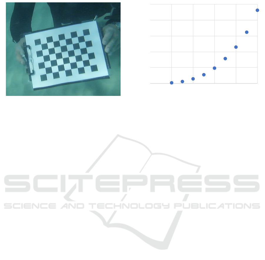
Figure 1: Sample target used for calibration. Here deployed
underwater.
sets to choose from. Clearly, a more structured ap-
proach is necessary to minimize this complex nature
of the problem.
Here we explore the application of a simple
RanSaC (Random Sample Consensus) (Fischler and
Bolles, 1981) algorithm to recruit appropriate stereo
image sets and compare this approach against re-
peated random sampling of the calibration image sets.
We demonstrate that given a fixed computational bud-
get RanSac provides an effective strategy for choosing
the calibration frame set.
The remainder of this paper is organized as fol-
lows. Section 2 introduces the basic problem. Sec-
tion 3 describes the simple RanSac approach used
here. This approach is compared against multiple
random calibrations of different calibration set sizes
in Section 4. Finally, Section 5 summarizes the ap-
proach and suggests extensions to the work.
2 BACKGROUND
There exist a number of standard computer vision li-
braries, and OpenCV is representative. The OpenCV
implementation of camera calibration is based on the
Matlab calibration code and relies on Zhang’s al-
gorithm (Zhang, 2000) for calibration. Although a
large number of options exist within both the OpenCV
and Matlab libraries, the basic task for stereo cam-
era calibration is typically structured as calibrating
the two cameras separately and then solving for the
camera separation geometry. Indeed, this is the ba-
sic approach suggested in the OpenCV documenta-
tion. Both the stereo camera separation and individ-
ual camera calibration processes are, in the Zhang
algorithm-based codebase, based on a planar calibra-
tion target of m calibration points (Figure 1) and the
0
5
10
15
20
25
0 10 20 30 40 50
Figure 2: Computational cost of calibrating a monocular
camera using the OpenCV camera calibration tool. Horiz-
tonal axis is the number of camera frames in the calibration
set. Vertical axis is the execution time in seconds. See text
for details of the hardware/software environment.
use of n such targets. The monocular camera calibra-
tion process of Zhang’s algorithm is based on mini-
mizing the error between the projection of each of the
n ×m calibration points and their projection using the
camera calibration, Specifically, to minimize
n
∑
I=1
m
∑
j=1
||m
i, j
− ˆm(A, R
i
,t
i
, M
j
)||
2
(1)
where m
i, j
are the calibration points, ˆm(A, R
i
,t
i
, M
j
) is
the estimation of the position of the calibration point
resulting from the calibration process. (R
i
, t
i
) defines
the rotation and position of the i’th camera, and M
j
is the j’th calibration point. This is a non-linear op-
timization process that iterates its optimization until
either a performance tolerance is obtained or a maxi-
mum number of interactions are performed. The crit-
ical observation here is that the number of iterations,
and thus the computational cost/time, increases with
the number of images in the calibration set.
To illustrate the effects of this, Figure 2 plots
the computational cost of just the camera calibration
stage (not including computing the location of the
calibration corner points) for calibrating a monocular
camera using OpenCV for calibration set sizes rang-
ing from 10 to 50. Each calibration set was run ten
times. Means and standard errors are plotted. The
implementation was in Python3 running on a 16GB
Apple M1 computer. Increasing set size results in a
superlinear increase in computational cost.
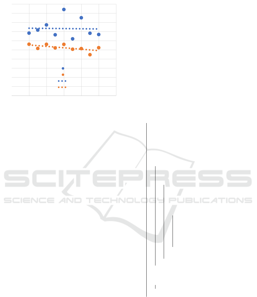
Increasing the size of the calibration set does not
necessarily improve calibration performance. This is
illustrated in Figure 3 which shows mean and max-
imum error for randomly chosen calibration target
sets. Each data point reflects ten calibration efforts of
a given calibration set size. Although the mean cali-
Stereo Video Camera Calibration in the Wild
65

0
0.1
0.2
0.3
0.4
0.5
0.6
0.7
0.8
0.9
1
0 10 20 30 40 50 60
Maximum Error
Mean Error
Linear (Maximum Error)
Linear (Mean Error)
Figure 3: Mean and maximum RMS reprojection error for
a monocular camera. Each data point corresponds to ten
randomly chosen calibration target images. The horizontal
axis shows the number of frames in the calibration set while
the vertical axis is the re-projection error (in pixels). As
the calibration set size increases the mean error decreases,
although the maximum error does not.
bration error decreases with increasing calibration set
size, the maximum error increases with increasing set
size. This illustrates the sensitivity of the calibration
process to outliers in the calibration frame set.
Selecting an appropriate calibration set in the wild
is complicated by difficulties associated with select-
ing the appropriate set of frames and computational
and calibration performance issues associated with
just selecting a large set of frames for calibration.
3 SELECTING A STEREO
CALIBRATION SET
The fundamental problem in calibrating a stereo video
dataset in the wild is that the nature of the data collec-
tion process prevents the controlled selection of im-
ages of the calibration target. (This problem can also
be found in monocular camera calibration, but here
we concentrate on the stereo version of the problem.)
We assume a set of N stereo images of the calibration
target and that for each of these N stereo image pairs
the target is properly captured in at least one of the
left and right images of the target. We also assume
that N ≫ 0.
The basic problem in choosing a good set of image
pairs is addressed using a greedy/RanSaC approach.
The algorithm is applied to the left and right image
sets to calibrate each camera separately. A final appli-
cation of the algorithm is used to obtain the geometry
between the two cameras. In each application of the
algorithm, a small initial set of frames is selected, and
additional stereo frames are added randomly to the set
of frames as long as this reduces the RMS reprojec-
tion error of the set. This process is repeated a number
of times and the best set of all of the frame sets iden-
tified is retained. The basic algorithm is sketched in
Algorithm 1.
input : S Initial set size, N maximum number
of attempts to find a good calibration
set, M maximum number of pairs to
add to S, L maximum number of
attempts to increase the set size before
failure
output: bestModel the best set of calibration
frames
bestModel ← None
i ← 0
while i < N do
Initialize the calibration model by selecting
S valid frames. This becomes the initial
inlier set while the remaining frames
becomes the initial outlier set.
j ← 0
success ← True
while j < M and success do
success ← False
k ← 0
while k < L and not success do
Choose a random frame x from the
outlier set. Compute MSE based
on inlier ∪ {x}.
if The MSE reduces relative to the
MSE of the inlier set then
Add x to the inlier set.
Remove x from the outlier set
Update the calibration model
with the new inlier set.
success ← True
end
k ← k + 1
end
end
if bestModel = None or model is better
than bestModel then
bestModel ← model
end
end
Algorithm 1: Greedy/RanSaC stereo camera calibration.
This process is run separately for the left and right image
views using the valid set of left and right calibration im-
ages. The process is then repeated on the valid set of cali-
bration images that provide both left and right views of the
calibration target to obtain the geometry between the two
cameras.
ICINCO 2023 - 20th International Conference on Informatics in Control, Automation and Robotics
66

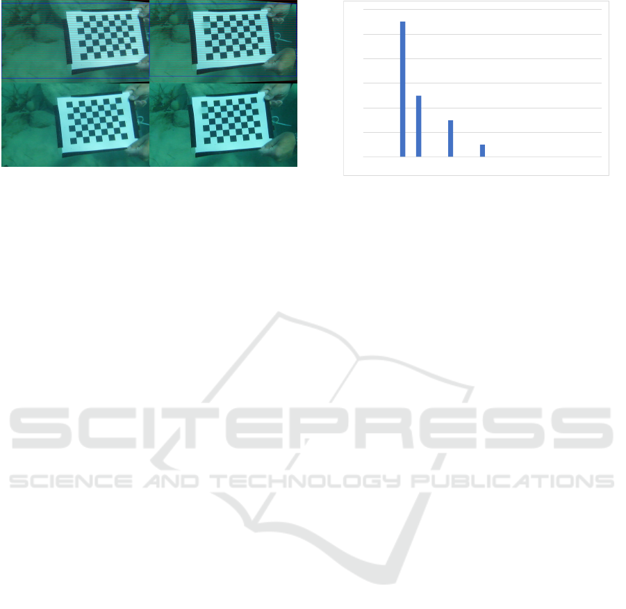
Figure 4: Sample calibration results from the RanSac-based
frame selection algorithm. The bottom row shows one im-
age pair from the input data stream, while the upper row
shows that same pair after rectification following calibra-
tion. The rectified image shows the calibration region of in-
terest (ROI) as well as overlaying horizontal lines showing
that the calibration has resulted in corresponding features
being aligned vertically.
In a traditional RanSaC algorithm the process of
adding elements to the inlier set will also be accompa-
nied by a process that removes outliers detected dur-
ing the process from the inlier set. Here we avoid
culling outliers from the set as we only add elements
to the inlier set if they reduce the RMS error and we
are particularly interested in having a range of differ-
ent views in the calibration set.
In obtaining a valid set of stereo calibration frames
we first process both the left and right images in each
pair to obtain calibration points. Frames that do not
obtain a valid left or right image of the calibration
target are discarded. The set of valid left and valid
right frames are used independently when selecting
frames for the left and right cameras. This maximizes
the set of possible frames for each camera. The set of
frames with both left and right calibration images are
used to calibrate the geometry between the cameras.
4 EVALUATION
In order to evaluate the stereo frame calibration al-
gorithm we utilized a dataset of stereo video frames
captured as part of a study of stereo video reconstruc-
tion of underwater structures. Data was collected us-
ing a Fuji W3 stereo camera in a custom underwa-
ter housing. Data was collected at 720p resolution.
A standard OpenCV calibration target (see Figure 1)
was used for calibration. As data was collected under-
water at depth, accurate camera control was difficult.
Surge moved both the camera operator and the target
resulting in poor control of the camera during data
collection.
0
2
4
6
8
10
12
0.2 0.4 0.6 0.8 1 1.2 1.4 1.6 1.8 2 2.2 2.4 2.6 2.8 3
Figure 5: Histogram of stereo video calibration errors using
Algorithm 1 from a single calibration sequence.
In order to explore the likely performance of Al-
gorithm 1, the algorithm was used to calibrate the
stereo camera with N = 5, S = 15, M = 10 and L = 5
using a single calibration dataset. Calibration was
performed 20 times with a mean calibration time of
approximately 240 seconds using the same hardware
and software environment as described above. The
mean calibration RMS error obtained with these pa-
rameters was 0.673 pixels. Results are plotted in Fig-
ure 5.
In order to evaluate the performance of Algo-
rithm 1 against a random selection of stereo calibra-
tion frames, a version of the stereo video calibration
framework was constructed that choose n
l
random
image frames to calibrate the left camera, n
r
random
frames to calibrate the right camera, and s random
stereo frames to calibrate the relationship between the
two cameras. Average running time of this baseline
with n
l
= n
r
= s took approximately 1.5 seconds (for
s = 15 frames), 7.12 seconds (for s = 25 frames) and
22 seconds (for s = 35 frames) to complete. Using the
time taken for one run of Algorithm 1 with the param-
eters described earlier as a computational budget, one
could perform almost 160 (s = 15), 34 (s = 25) or 11
(s = 35) efforts at calibrating the stereo camera pair
using a random set of images using the same compu-
tational budget. Given a specific computational time
budget, is it more effective to use the greedy RanSaC
algorithm given in Algorithm 1 or to run calibration
with random selections of frames of a given frame set
size?
In order to explore this we used eleven differ-
ent calibration sessions of the same underwater target
shown in Figure 1 collected over a week off the west-
ern coast of Barbados. Calibration took place from
3m to 8m below the surface using the same Fuji W3
stereo camera as described earlier. Data was collected
using a three-person diver team. One operating the
camera, one operating the calibration target and one
safety diver.
Stereo Video Camera Calibration in the Wild
67

[0.4, 0.6]
(0.6, 0.9]
(0.9, 1.1]
(1.1, 1.3]
(1.3, 1.6]
(1.6, 1.8]
(1.8, 2.1]
(2.1, 2.3]
(2.3, 2.5]
(2.5, 2.8]
(2.8, 3.0]
0
100
200
300
400
500
600
700
800
900
1000
(a) 15
[0.4, 0.6]
(0.6, 0.9]
(0.9, 1.1]
(1.1, 1.4]
(1.4, 1.6]
(1.6, 1.8]
(1.8, 2.1]
(2.1, 2.3]
(2.3, 2.5]
(2.5, 2.8]
(2.8, 3.0]
0
50
100
150
200
250
(b) 25
[0.4, 0.7]
(0.7, 0.9]
(0.9, 1.1]
(1.1, 1.4]
(1.4, 1.6]
(1.6, 1.8]
(1.8, 2.1]
(2.1, 2.3]
(2.3, 2.5]
(2.5, 2.8]
(2.8, 3.0]
0
10
20
30
40
50
60
70
(c) 35
Figure 6: Histogram of stereo video calibration errors using
the random frame strategy with different sized frame sets.
Note that the right hand column in each graph includes all
data points to the right of the distribution shown.
For each calibration set a single video recording
was made, typically of 30-60 s in duration. For each
of the eleven calibration sequences Algorithm 1 was
run as were repeated calibration efforts using ran-
domly chosen set sizes of 15, 25 and 35 frames. The
set sizes were chosen to match the computational cost
of Algorithm 1; 160 (s = 15), 34 (s = 25), and 11
(s = 35). Table 1 and Figure 6 summarize the per-
formance of the RanSaC algorithm and the various
random algorithms run with the same time budget.
A random calibration approach was said to fail if it
produced a RMS reprojection error of three pixels or
more. This corresponds to the right most column in
Figure 6.
Note that choosing a larger calibration set size
does not necessarily result in an improvement in the
resulting calibration. Choosing a RMS of three or
higher as failure, then 43% of the random efforts re-
sult in failure with s = 15, 33% with s = 25 and 41%
with s = 35. Although low RMS values are associated
with smaller set sizes, such low sampling is unlikely
to capture the full viewing space of the calibration tar-
get.
Although repeated random selection of calibration
sets can produce a “good” calibration, and indeed out-
perform Algorithm 1, it also results in a number of
calibrations that fail.
It is interesting to note that although the same
camera calibration target, camera and underwater
housing, and dive team were used for each of the data
collection sessions there is a wide range of calibration
performance results. Some data sessions (e.g., 1886)
have relatively poor calibration performance across
all of the algorithms tested, while in other sessions
(e.g., 1895) each of the algorithms provided accept-
able results, at least when choosing the ‘best’ error
from the calibration set.
5 DISCUSSION
Calibrating a stereo camera rig in the wild introduces
a range of issues that are not normally found under
laboratory conditions. The underwater condition is
perhaps the most challenging. Communication be-
tween individuals performing the calibration is dif-
ficult as is control of the calibration target and the
imaging stereo rig. Nor is it straightforward to accu-
rately monitor the camera capture process. Underwa-
ter camera viewfinders can be difficult to view when
wearing SCUBA equipment, and it can be difficult or
impossible to view both left and right camera views in
real time. As a consequence, highly controlled imag-
ing of the calibration target is not possible. Instead,
a common approach is to collect a large amount of
calibration data and then to choose which frames to
process upon return to the lab. As ground truth of
the calibration set – where the camera rig was rela-
tive to the calibration target – is not easily obtained,
this selection process must operate in a poorly or un-
informed manner. Here we have demonstrated that a
greedy RanSac approach can produce calibration im-
age sets that lead to good camera calibration. We also
demonstrate that although the computational budget
ICINCO 2023 - 20th International Conference on Informatics in Control, Automation and Robotics
68

Table 1: RanSac performance against random for multiple calibration datasets. ID is an identification number assigned to
each set. Valid Frames refers to the number of frames in the dataset that gave rise to valid left (L), right (R) or stereo (S)
images of the calibration target. RanSac RMS is the RMS projection error for one run of Algorithm 1, while Best, Mean and
Fails are the best and mean RMS values for the Random Algorithm while Fails is the percentage of calibration efforts that
resulted in a RMS error of three pixels or more. For some of the calibration sequences (e.g., 1886) random calibration sets
perform poorly over all three set sizes. While for others (e.g., 1906) smaller set sizes performed quite well almost always.
ID Valid Frames RanSac Random 15 Random 25 Random 35
L R S RMS Best Mean Fails Best Mean Fails Best Mean Fails
1886 689 680 680 8.48 1.14 35.3 96% 1.52 39.2 97% 2.14 31.5 90%
1887 768 744 744 2.06 0.63 18.1 56% 0.82 22.5 51% 0.81 20.9 72%
1895 687 694 687 0.48 0.47 9.40 43% 0.73 12.8 48% 0.51 4.47 9%
1896 596 593 589 32.1 0.76 15.1 77% 1.20 15.3 82% 1.36 5.50 54%
1905 932 929 929 2.25 1.13 30.8 87% 1.36 40.3 94% 20.8 43.6 100%
1906 538 505 498 0.52 0.40 2.86 9% 0.41 1.90 6% 0.43 4.28 19%
1915 636 636 636 5.40 0.74 13.7 89% 1.09 11.7 67% 1.46 21.3 81%
1916 736 733 733 1.15 0.65 12.3 39% 0.70 15.5 61% 0.72 20.8 72%
1923 402 401 401 1.98 0.82 2.29 16% 0.88 1.87 9% 1.01 1.86 18%
1940 217 225 213 0.44 0.42 16.0 29% 0.46 19.0 42% 0.44 12.16 27%
1941 469 497 468 1.08 0.84 4.92 19% 0.96 6.86 27% 1.13 3.23 9%
to obtain these sets could be used to choose multiple
sets of different sizes and then to just “take the best”
resulting set, this approach is not guaranteed to pro-
duce a good set of views. Rather, many of these cal-
ibration efforts will produce camera calibrations that
produce RMS errors much greater than three pixels.
An error that will lead to stereo misalignment or sig-
nificant error in recovered scene structure.
All that being said, in practice the calibration pro-
cess in the lab has the advantage of providing for the
calibration process to be run repeatedly until accept-
able calibration performance results. We have found
that a RanSaC greedy approach can be used to focus
such repeated searches for a good calibration set in a
way that does not require a predetermined calibration
set size and which can use a greedy approach to se-
lect elements of the calibration set so as to optimize
the RMS reprojection error.
The RanSaC algorithm (Algorithm 1) works to
minimize the projection error. This is not the only er-
ror metric that might be used. For example, it would
be possible to construct an error that not only sought
to minimize the reprojection error but at the same time
seeks to maximize the size of the calibration image
set, or the distribution of camera poses used for cali-
bration. This is the subject of ongoing investigation.
ACKNOWLEDGEMENTS
The financial support of the NCRN and NSERC
Canada is greatfully acknowledged.
REFERENCES
Engel, J., St
¨
uckler, J., and Cremers, D. (2015). Large-scale
direct SLAM with stereo cameras. In IEEE/RSJ In-
ternational Conference on Intelligent Robots and Sys-
tems (IROS), pages 1935–1942, Hamburg, Germany.
Fischler, M. A. and Bolles, R. C. (1981). Random sample
consensus: A paradigm for model fitting with appli-
cations to image analysis and automated cartography.
Commun. ACM, 24(6):381–395.
Hartley, R. and Zisserman, A. (2003). Multiple View Geom-
etry in Computer Vision. Cambridge University Press.
Pollefeys, M., Nist
´
er, D., Frahm, J.-M., Akbarzadeh, A.,
Mordohai, P., Clipp, B., Engels, C., Gallup, D., Kim,
S.-J., Merrell, P., et al. (2008). Detailed real-time ur-
ban 3d reconstruction from video. International Jour-
nal of Computer Vision, 78(2-3):143–167.
Poulin-Girard, A.-S., Thibault, S., and Laurendeau, D.
(2016). Influence of camera calibration conditions
on the accuracy of 3d reconstruction. Optics express,
24(3):2678–2686.
Salvi, J., Armangu
´
e, X., and Batlle, J. (2002). A compar-
ative review of camera calibrating methods with ac-
curacy evaluation. Pattern recognition, 35(7):1617–
1635.
Torr, P. H. and Zisserman, A. (2000). Mlesac: A new ro-
bust estimator with application to estimating image
geometry. Computer vision and image understanding,
78(1):138–156.
Zhang, Z. (2000). A flexible new technique for camera cal-
ibration. IEEE Transactions on Pattern Analysis and
Machine Intelligence (PAMI), 22:1330–1334.
Zhang, Z., Deriche, R., Faugeras, O., and Luong, Q.-T.
(1995). A robust technique for matching two uncal-
ibrated images through the recovery of the unknown
epipolar geometry. Artificial intelligence, 78(1-2):87–
119.
Stereo Video Camera Calibration in the Wild
69