
Modelling of a 6DoF Robot with Integration of a Controller Structure
for Investigating Trajectories and Kinematic Parameters
Armin Schleinitz, Chris Schöberlein
a
, Andre Sewohl
b
, Holger Schlegel and Martin Dix
c
Institute for Machine Tools and Production Processes, Chemnitz University of Technology,
Reichenhainer Str. 70, 09126 Chemnitz, Germany
Keywords: Robotic, Simulation, Kinematic Analyse, Inverse Transformation, Multi-Body Modelling, Feedback Control
System.
Abstract: Knowledge of robot joint position as a function of TCP-position and pose is of outstanding importance, since
position and pose are specified by the process. However, there is no generally applicable method for the
inverse transformation. In addition to a kinematic analysis and the inverse transformation of a 6DoF robot,
this work also presents the development of a multi-body model based on it. All components are linked in a
drive-specific controller structure. To validate the overall model, the simulation-based drive torques are
compared with the values of a real robot. Likewise, target and actual Tool Center Point (TCP) positions of a
given trajectory are examined in the simulation model and compared with a real system. It was shown that in
the simulation model, the realized trajectory exhibits only very slight deviations compared to the previous
trajectory, but greater deviations compared to the real system. The overall model forms the basis for further
analyses regarding kinematic joint parameters as a function of a given trajectory.
1 INTRODUCTION
Robots are conquering more and more areas of
application in industrial production. They are not only
used in component handling, in joining and assembly
operations. For some time, the possibilities of using
robots in cutting machining have also been
investigated (Abele et al. 2008). However, numerous
challenges still need to be overcome in this area in
order to further expand the range of applications. In
this context, a wide range of work and investigations
have already been carried out, which aim to increase
the rigidity (Lin et al. 2017) and the movement
speeds, but also to increase the positioning,
repeatability and path accuracy (Hu et al. 2023). The
optimization approaches pursued for this essentially
concentrate on the following subject areas:
- Stiffness modelling and pose planning
- Identification of dymanic parameters and
trajectory planning
- Compensation of structural deformation
a
https://orcid.org/0009-0006-3603-5012
b
https://orcid.org/0000-0003-2031-6603
c
https://orcid.org/0000-0002-2344-1656
- Analysis of vibration characteristics and chatter
suppression (Zhu et al. 2022).
One common feature of all approaches are
suitable simulation models for replicating the system
and process behaviour (Metzner et al. 2019). In this
paper, an approach is presented in which a multi-body
simulation model is developed based on the kinematic
analysis and the inverse transformation. Knowledge
of robot joint position as a function of TCP-position
and pose is of outstanding importance, since position
and orientation are specified by the process.
Compared to the forward transformation, however,
the inverse or backward transformation for an open
kinematic chain is much more complicated. However,
there is no generally applicable method that can be
applied to all types of robots. This paper presents the
application of a geometric approach for the inverse
transformation in the simulation model. This is
subdivided in two problems: the special backward
calculation for determining joint angles one to three
as well as the explicit backward calculation for joint
Schleinitz, A., Schöberlein, C., Sewohl, A., Schlegel, H. and Dix, M.
Modelling of a 6DoF Robot with Integration of a Controller Structure for Investigating Trajectories and Kinematic Parameters.
DOI: 10.5220/0012203700003543
In Proceedings of the 20th International Conference on Informatics in Control, Automation and Robotics (ICINCO 2023) - Volume 1, pages 697-703
ISBN: 978-989-758-670-5; ISSN: 2184-2809
Copyright © 2023 by SCITEPRESS – Science and Technology Publications, Lda. Under CC license (CC BY-NC-ND 4.0)
697
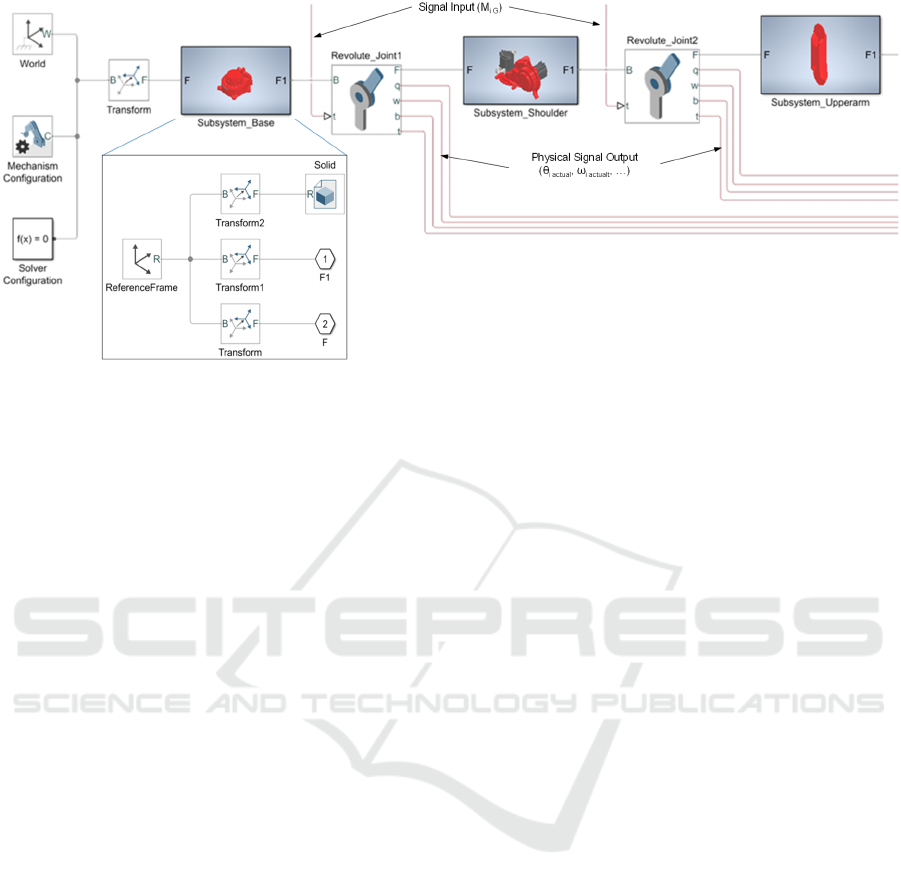
Figure 1: Structure of the Multi-Body model designed in MatLab-Simulink
®
.
angles four to six (Siegert, 1996). In Addition, the
model is connected to a drive-specific controller
structure in MatLab-Simulink
®
. This combination
enables the investigation of robot behaviour and
kinematic joint parameters depending on a given
trajectory and the overall model forms the basis for
further analyses in future.
2 MODEL DEVELOPMENT
2.1 Multi-Body Model
Initially, it is necessary to create the physical robot
structure in MatLab. The model is based on a Comau
NJ130 2.05 robot created with aid of MatLab-
Simcape
®
. The overall structure is shown in Fig. 1.
First of all, the global coordinate system (World
Frame) to which the model is aligned has to be
defined. For this purpose, a function block is
generated which, among other things, reflects the
value and the direction of the prevailing gravity
(Mechanism Configurator). In addition, a solver
(Solver Configuration) must be specified. These three
function blocks are connected with a Rigid Transform
function block, which enables a manipulation of the
alignment of the connected structures.
The Rigid Transform function block is followed
by a subsystem that contains the structure for the first
link (robot foot). Each subsystem has two ports that
form the physical connection to the neighbouring
elements. In each subsystem, a Rigid Transform
function block is set after or before each port. This
allows the geometric robot structure to be taken into
account. The translational and rotational
specifications define the connection points for
neighbouring elements. These are aligned in such a
way that they correspond to the Denavit &
Hartenberg nomenclature (DH nomenclature) (cf.
table 1). Likewise, at least one solid (File Solid) is
modeled in a subsystem and connected to the existing
structure with a Rigid Transform function block. With
the File Solid function block, geometry, material and
visual properties can loaded an external file into the
model. Masses and centers of gravity of the solids can
also be defined and included in the model. It is also
possible to insert a Reverence Frame in each
subsystem.
In the robot’s kinematic chain, the Robot base
subsystem is followed by a revolute joint. For
modelling, a Revolute Joint function block is used
whose axis of rotation is always oriented in the z-
direction as a consequence of the arrangement of the
Rigid Transform function block at the ports of the
subsystems. Likewise, the upper and lower limits are
specified in the rotary joint according to the robot data
sheet (Comau, 2023). However, further properties
can be added to the revolute joint. They serve as
actuators to which a torque can be applied. At the
same time, Revolute Joint function blocks can serve
as sensors and provide angular position and velocity
via physical signal ports. For further modelling of the
robot, another subsystem (robot shoulder) is
connected to the second port of the revolute joint (F).
According to this procedure, the entire kinematic
chain of the robot is built up.
2.2 Controller Structure
In order to move the created robot structure in a
targeted manner, it is necessary as a further step to
model a corresponding controller structure for the six
ICINCO 2023 - 20th International Conference on Informatics in Control, Automation and Robotics
698

Figure 2: Signal diagram of the position control with
simplified speed control loop.
axes. For this purpose, a controller structure is created
in MatLab-Simulink
®
. The design required for the
simulation follows the explanations of GROß,
HAMANN, WIEGÄRTNER (cf. Groß, 2006). The
authors describe the creation of a simplified speed
control loop in which the current control loop is
included in the sum of the small delay times of the
speed control loop (T
σn
) For this purpose, the
substitute structure and its setting variables are
determined for the speed control loop. In the further
course, the controller structure is extended by a
superimposed position control loop. The model thus
follows a cascade structure (cf. figure 2).
For the calculation of suitable controller
parameters, specific variables of the drives and the
servo inverters must be included. Drive RA1 is used
as an example to describe the parameterization (cf.
table 1).
Table 1: Controller Parameters (RA1).
Parameter Name Sign Value
Sample time current
loo
p
T
Ai
125e-6 s
Sample time speed
control loo
p
T
An
125e-6 s
Sampling time
p
osition control loop
T
Ax
4000e-6 s
Motor constant
K
m
1.23 Nm/A
As already mentioned, the calculation of the
controller parameters follows the explanations of
GROß, HAMANN AND WIEGÄRTNER (cf. Groß,
2006) and takes into account the optimization rule of
the symmetrical optimum. A high damping (0.707)
was assumed for the determination of the equivalent
time constant in the speed control loop system (
T
En
).
This means that there is a sufficiently large phase
reserve, which represents a criterion for controller
stability. Likewise, for the calculation of the gain
factor in the position controller (K
v
), a significantly
higher damping has been assumed, taking into
account formula 1. This leads to a lower K
V
value and
consequently to a reduced overshoot. All determined
controller parameters for drive 1 are listed in table 2.
This procedure is carried out analogously for all
six drives. Equal sampling times are used while motor
constants are adjusted according to data sheets.
𝐾
1
2∗𝑇
(1)
Table 2: Controller Parameters (RA1).
Controller parameter Sign Value
Equivalent time constant of
current control loop
T
Ei
3.6e-04 s
Equivalent time constant speed
control loop
T
En
0.0012 s
Sum of the small time constants of
the s
p
eed control loo
p
T
N
6.1e-04 s
Gain factor speed controller K
P
6.3934
Nms/ra
d
Equivalent delay time of the speed
control loop
T
n
0.0024 s
Speed setpoint delay time T
Gn
0.0024 s
Sum of the small time constants of
the
p
osition control loop
T
x
0.0096 s
Gain factor position controller K
v
0.5210 s
-1
3 TRANSFORMATIONS
3.1 Forward Transformation
The Comau NJ130 2.05 is a 6-DoF robot whose
structure as well as position and orientation of the
coordinate systems of the axes are shown in figure 3
(Comau, 2023). In order to describe the robot
kinematics unambiguously in mathematical terms,
the DH convention has been established (Denavit and
Hartenberg, 1955). The parameters for the robot used
are listed in table 3.
Figure 3: Comau NJ130 2.05.
Modelling of a 6DoF Robot with Integration of a Controller Structure for Investigating Trajectories and Kinematic Parameters
699

Table 3: DH-Parameters for Comau NJ130 2.05.
Link θ
i
a
i
[m] d
i
[m] α
i
[°]
1 var 0.40 0.55 -1.570796
2 var 0.86 0 0
3 var 0.21 0 -1.570796
4 var 0 0.7615773 1.570796
5 var 0 0 -1.570796
6 var 0 0.21 0
The six linked axes are described by four DH
parameters joint angle (θ
i
), arm lengh (a
i
), joint offset
(d
i
) and torsion angle (α
i
) (Mareczek, 2020a).
Furthermore, axis-specific rotational and
translational transformation matrices leads to form
the general A-matrix according to formula 2.
A
cos𝜃
sin𝜃
cos𝛼
sin𝜃
sin𝛼
𝑎
cos𝜃
sin𝜃
cos𝜃
cos𝛼
cos𝜃
sin𝛼
𝑎
sin𝜃
0sin𝛼
cos𝛼
𝑑
00 01
(2)
Knowing all joint positions and DH parameters as
well as the calculation by means of the A-matrix, the
position of the TCP with respect to the robot base,
which at the same time represents the base coordinate
system, can be calculated according to formula 3.
T
A
A
∗
A
∗
A
∗
A
∗
A
∗
A
(3)
3.2 Inverse Transformation
For practical use, however, knowledge of robot joint
position as a function of TCP-position and pose is of
outstanding importance, since position and pose are
specified by the process. Compared to the forward
transformation, however, the inverse or backward
transformation for an open kinematic chain is much
more complicated. There is no generally applicable
method for this. The basic solution approaches are
divided into algebraic, numerical and geometric
methods (Goldenberg et al. 1985). In the present
model, the inverse transformation is solved using a
geometric approach, which assumes that joint axes
four to six intersect at the wrist root (S4) (Siegert,
1996). The overall approach is subdivided of two
subproblems: the special backward calculation for
determining joint angles one to three as well as the
explicit backward calculation for joint angles four to
six. The wrist position of the robot is defined by the
first partial solution and orientation of the end
effector by the second partial solution. In addition, to
obtain a unique solution, three configuration
parameters (ARM, ELBOW, FLIP) were selected
depending on the existing configuration (cf. Siegert,
1996).
For the special inverse calculation, knowledge of
carpus position (S4) is decisive which is calculated
from:
𝑆4
𝑝
𝑝
𝑝
𝑝
𝑝
𝑝
𝑑
∗
𝑎
𝑎
𝑎
(4)
From knowledge of S4, its projection on the x
0
- y
0
surface results as S4’. With this relationship, joint
angle θ
1
can now be determined as function of the
present robot configuration:
𝜃
𝑎𝑟𝑐𝑡𝑎𝑛2
𝐴
𝑅𝑀 ∗𝑝
;
𝐴
𝑅𝑀 ∗𝑝
(5)
Now, to determine the joint angle θ
2
, a
1
and d
1
must be taken into account, so that only the position
between S1 to S4 is considered:
𝑞
𝑝
𝑝
𝑝
𝑝
𝑝
𝑝
𝑎
𝑎
𝑑
∗
𝑐𝑜𝑠
𝜃
𝑠𝑖𝑛𝜃
1
(6)
Knowing q' and R', relationships for the auxiliary
angles sin(α) and cos(α) as well as for sin(β) and
cos(α) can be derived (cf. figure 4). Taking into
account the robot configuration parameters ARM and
ELBOW as well as the addition theorem for angular
functions, one obtains the following equations:
Figure 4: Comau NJ130 2.05 with angular relations.
ICINCO 2023 - 20th International Conference on Informatics in Control, Automation and Robotics
700
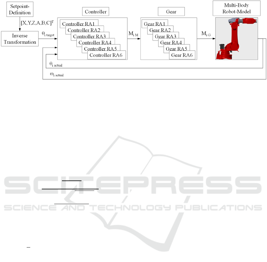
Figure 5: Simulation model.
𝑠𝑖𝑛
𝜃
𝑠𝑖𝑛
𝛼
∗𝑐𝑜𝑠
𝛽
𝐸𝐿𝐵𝑂𝑊∗
𝑐𝑜𝑠
𝛼
∗𝑠𝑖𝑛
𝛽
(7)
cos
𝜃
𝐴
𝑅𝑀∗ 𝑐𝑜𝑠
𝛼
∗ cos
𝛽
𝐴
𝑅𝑀∗
𝐸𝐿𝐵𝑂𝑊∗ 𝑠𝑖𝑛
𝛼
∗sin
𝛽
(8)
Using the arctangent-2 function, this determines
the joint angle θ
2
.
𝜃
𝑎𝑟𝑐𝑡𝑎𝑛2𝑠𝑖𝑛
𝜃
;cos
𝜃
(9)
To calculate joint angle θ
3
, the auxiliary angle ψ
is initially determined from:
𝑐𝑜𝑠
𝜓
𝑎
𝑎
𝑑
𝑞
2 ∗ 𝑎
∗𝑎
𝑑
(10)
sin
𝜓
1
cos
𝜓
(11)
Applying the arctangent-2 function again, the
auxiliary angle ψ is obtained. This is inserted into the
following formula, which calculates joint angle θ
3
.
𝜃
𝜋
2
𝐴
𝑅𝑀∗𝐸𝐿𝐵𝑂𝑊∗𝜓𝜋
(12)
The Explicit-Backward-Calculation is described
in (Siegert, 1996) and can be applied to this robot
considering the present DH parameters.
3.3 Overall Model
Eventually an overall model is created from the
modeled components (cf. figure 5). It contains the
multi-body robot model, which is connected to the
control structure. Thus, the actual joint angle position
(θ
i actual
) and the actual joint angle velocity (ω
i actual
) are
fed back into the control structure. In addition, a
setpoint generator and gear stages between controller
and robot complete the model. Hence, it is possible to
specify the setpoint position (X,Y,Z) as well as the
pose (A,B,C) as angle information in the global
coordinate system continuously in time. The target
values are converted into corresponding joint angles
(θ
i target
) by means of inverse transformation and
transferred to the controller. The axis-specific
controllers determine the joint angle deviation and
balance them out.
4 RESULTS
To verify the Simscape multi-body model, it is
possible to specify the corresponding joint angles
directly. If these joint angles are all set equal to "0",
the robot position from figure 3 is obtained. This
position is described in the manual (Comau, 2023)
and leads to a TCP of
P0 = [1.37158 0 1.62 0 1.5708 0]
T
considering the
described DH parameters. The model leads to the
identical TCP.
To check the inverse transformation, P0 is used as
a setpoint specification. Inverse transformation
should determine the corresponding joint angles. The
TCP-resulting from the simulation model is identical
to the specified point P0.
To derive meaningful conclusions, it is necessary
to compare the model with the real system. For this
purpose, a real Comau NJ130 2.05 robot is available
for comparative tests. The aim is to keep the
deviations between the model and the real system as
small as possible with regard to the subsequent
focused points of the investigation.
First, a static consideration of joint-specific
torques (M
i M
) at input of the transmission using TCP
position P0 is carried out. Table 4 compares the joint-
specific holding torques for the TCP position. All
deviations are neglectable small and can be explained
by simplifications of the model. For example, friction
and damping in the gears and joints have not been
considered.
Modelling of a 6DoF Robot with Integration of a Controller Structure for Investigating Trajectories and Kinematic Parameters
701
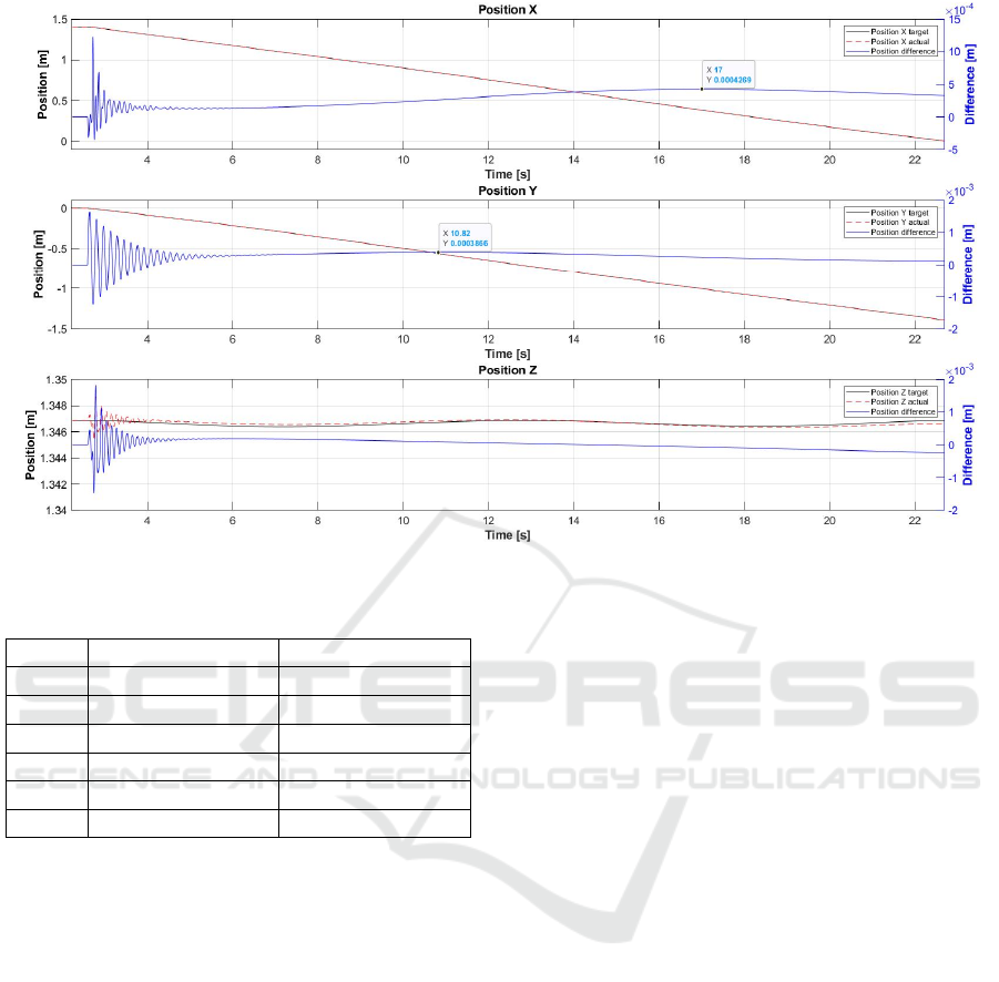
Figure 6: TCP-Position of the simulation-model (P1 to P2).
Table 4: Motor Torque [Nm] on P0.
Jerk Simulation Comau NJ130 2.05
1 0 0.1
2 -6 -5.89
3 -5.741 -5.94
4 0 0
5 -1.572 -1.52
6 0 0.02
By means of setpoint specification and inverse
transformation, a motion execution is possible. The
simulation model was given a trajectory which leads
directly from P1 = [1.3975 0 1.3469 0 1.5708 0]
T
to
P2 = [0 1.3975 1.346 0 1.5708 1.5708]
T
. The TCP-
curves of the setpoint specification and the realized
trajectory are shown in figure 6. Only small
deviations of the two curves can be seen. In
X-direction as well as in Y-direction 0.3 mm each.
However, the oscillations at the beginning of the
movement are particularly noticeable. These
originate from the actual curve and should be quickly
compensated by the corresponding controllers. It
must be taken into account that overshooting is
problematic in robotics, since it can lead to collisions
of the robot with the environment (Mareczek, J.,
2020b). Regardless of this, the occurrence of this
transient behavior is an indication of insufficient
regulation of the system.
Figure 7 shows the comparison of the TCP-
position of the trajectories between the simulation
model and the real system. Only the actual trajectories
are considered, which again lead on a direct path from
P1 to P2. During this movement, θ
1
must rotate by
-90°. First of all, it can be stated that deviations of the
given trajectory between simulation model and real
system are recognizable, the maximum of which is
amount to 19.61 mm for position X, 15.68 mm for
position Y and 1 mm for position Z. It is striking that
the largest deviations between the two trajectories
occur between 0° and -45° and between -45° and
-90°. Taking into account the small deviations
between target and actual positions from the
simulation model (cf. figure 6), only the desired value
generation or the inverse transformation can be
considered as the cause and therefore should be
optimized for further investigations.
5 SUMMARY AND OUTLOOK
For a 6-DoF robot (Comau NJ130 2.05), the DH
convention was used to show the forward
transformation. The inverse transformation was
solved with a geometric approach. Hence, the inverse
transformation is devided into two subproblems, the
special and the explicit inverse. A simulation model
was created in which both transformations were
linked with a multi-body model and supplemented by
an axis-specific controller structure. With this
approach for the inverse transformation, a suitable
ICINCO 2023 - 20th International Conference on Informatics in Control, Automation and Robotics
702

Figure 7: TCP-Position simulation model vs. real system (P1 to P2).
overall model was developed, which can form the
basis for further analysis regarding controller
parameters together with kinematic joint parameters
as a function of a given trajectory.
It was shown that the static holding torques at the
input to the gearbox are comparable between
simulation model and real system. It was also shown
that the realized trajectory in the simulation model
exhibited only very slight deviations compared to the
predefined trajectory. In comparison with a real
system, however, larger deviations were found.
At the start of the movement of the simulation
model, there are rigid oscillations which are only
slowly eliminated. Thus, the control system appears
to be insufficient. For this purpose, the controller
structure should be adapted by a more precise
modelling of the current, speed and position control
loop, resulting in a more complex controller cascade.
After optimizing the controller structure of the
individual joints, the overall model is ready for
further analysis. In particular, analyses with reference
to specific, predetermined trajectories and their
resulting kinematic parameters at the TCP and in the
joints become possible.
REFERENCES
Abele, E., Bauer, J., Rothenbücher, S. Stelzer, M., von Stryk,
O. (2008), Prediction of the Tool Displacement by
Coupled Models of the Compliant Industrial Robot and
the Milling Process, Proceedings of the International
Conference on Process Machine Interactions, pp. 223-
230.
Lin, Y., Zhao, H., Ding, H. (2017), Posture optimization
methodology of 6R industrial robots for machining using
performance evaluation indexes. Robotics and
Computer-Integrated Manufacturing, Volume 48,
pp. 59-72.
Hu, Y., Zhang, S., Chen, Y. (2023), Trajectory Planning
Method of 6-DOF Modular Manipulator Based on
Polynomial Interpolation, Journal of Computational
Methods in Sciences and Engineering, pp. 1-12.
Zhu, Z., Tang, X., Chen, C., Peng, F., Yan, R., Zhou, L., Li,
Z., Wu, J. (2022). High precision and efficiency robotic
milling of complex parts: Challenges, approaches and
trends. Chinese Journal of Aeronautics, Volume 35,
Issue 2.
Metzner, M., Weissert, S., Karlidag, E., Albrecht, F., Blank,
A., Mayr, A., Franke, J. (2019), Virtual Commissioning
of 6 DoF Pose Estimation and Robotic Bin Picking
Systems for Industrial Parts, IFAC-PapersOnLine,
pp. 160-164.
Groß, H., Hamann, J., Wiegärtner, G. (2006). Elektrische
Vorschubantriebe, Publicis Kommunikations Agentur
GmbH, GWA, Erlangen.
Denavit, J., Hartenberg, R.S. (1955). A Kinematic Notation
for Lower-Pair Mechanisms Based on Matrices. ASME
Journal of Applied Mechanics, 22, pp. 215-221.
Comau (2023), Comau_Nj13020_Workingareas, Comau
S.p.A., Grugliasco.
Mareczek, J. (2020a). Grundlagen der Roboter-
Manipulatoren – Band 1: Modellbildung von Kinematik
und Dynamik. Berlin: Springer Vieweg.
Goldenberg, A., Benhabib, B., Fenton, R. (1985). A complete
generalized solution to the inverse kinematics of robots,
IEEE Journal on Robotics and Automation, vol. 1, no. 1,
pp. 14-20.
Siegert, H. (1996). Robotik: Programmierung intelligenter
Roboter. Berlin: Springer.
Mareczek, J. (2020b). Grundlagen der Roboter-
Manipulatoren – Band 2: Pfad- und Bahnplanung,
Antriebsauslegung, Regelung. Berlin: Springer Vieweg.
Modelling of a 6DoF Robot with Integration of a Controller Structure for Investigating Trajectories and Kinematic Parameters
703
