Make Deep Networks Shallow Again
Bernhard Bermeitinger
a
, Tomas Hrycej and Siegfried Handschuh
b
Institute of Computer Science, University of St.Gallen (HSG), St.Gallen, Switzerland
Keywords:
Residual Connection, Deep Neural Network, Shallow Neural Network, Computer Vision, Image
Classification, Convolutional Networks.
Abstract:
Deep neural networks have a good success record and are thus viewed as the best architecture choice for com-
plex applications. Their main shortcoming has been, for a long time, the vanishing gradient which prevented
the numerical optimization algorithms from acceptable convergence. An important special case of network
architecture, frequently used in computer vision applications, consists of using a stack of layers of the same di-
mension. For this architecture, a breakthrough has been achieved by the concept of residual connections—an
identity mapping parallel to a conventional layer. This concept substantially alleviates the vanishing gradient
problem and is thus widely used. The focus of this paper is to show the possibility of substituting the deep
stack of residual layers with a shallow architecture with comparable expressive power and similarly good con-
vergence properties. A stack of residual layers can be expressed as an expansion of terms similar to the Taylor
expansion. This expansion suggests the possibility of truncating the higher-order terms and receiving an archi-
tecture consisting of a single broad layer composed of all initially stacked layers in parallel. In other words, a
sequential deep architecture is substituted by a parallel shallow one. Prompted by this theory, we investigated
the performance capabilities of the parallel architecture in comparison to the sequential one. The computer
vision datasets MNIST and CIFAR10 were used to train both architectures for a total of 6,912 combinations
of varying numbers of convolutional layers, numbers of filters, kernel sizes, and other meta parameters. Our
findings demonstrate a surprising equivalence between the deep (sequential) and shallow (parallel) architec-
tures. Both layouts produced similar results in terms of training and validation set loss. This discovery implies
that a wide, shallow architecture can potentially replace a deep network without sacrificing performance. Such
substitution has the potential to simplify network architectures, improve optimization efficiency, and acceler-
ate the training process.
1 INTRODUCTION
Deep neural networks (i.e., networks with many non-
linear layers) are widely considered to be the most
appropriate architecture for mapping complex depen-
dencies such as those arising in Artificial Intelligence
tasks. Their potential to map intricate dependencies
has advanced their widespread use.
For example, the study (Meir et al., 2023) com-
pares the first deep convolutional network for image
classification with two sequential convolutional lay-
ers LeNet (LeCun et al., 1989) to its deeper evolu-
tion VGG16 (Simonyan and Zisserman, 2015) with
13 sequential convolutional layers. While the perfor-
mance gain in this comparison was significant, fur-
ther increasing the depth resulted in very small per-
a
https://orcid.org/0000-0002-2524-1850
b
https://orcid.org/0000-0002-6195-9034
formance gains. Adding three additional convolu-
tional layers to VGG16 improved the validation error
slightly from 25.6 % to 25.5 % on the ILSVRC-2014
competition dataset (Russakovsky et al., 2015) while
increasing the number of trainable parameters from
138M to 144M.
However, training these networks remains a sig-
nificant challenge, often navigated through numeri-
cal optimization methods based on the gradient of the
loss function. In deeper networks, the gradient can
significantly diminish particularly for parameters dis-
tant from the output, leading to the well-documented
issue known as the “vanishing gradient”.
A breakthrough in this challenge is the concept of
residual connections: using an identity function par-
allel to a layer (He et al., 2016). Each residual layer
consists of an identity mapping copying the layer’s
input to its output and a conventional weighted layer
with a nonlinear activation function. This weighted
Bermeitinger, B., Hrycej, T. and Handschuh, S.
Make Deep Networks Shallow Again.
DOI: 10.5220/0012203800003598
In Proceedings of the 15th International Joint Conference on Knowledge Discovery, Knowledge Engineering and Knowledge Management (IC3K 2023) - Volume 1: KDIR, pages 339-346
ISBN: 978-989-758-671-2; ISSN: 2184-3228
Copyright © 2023 by SCITEPRESS – Science and Technology Publications, Lda. Under CC license (CC BY-NC-ND 4.0)
339

layer represents the residue after applying the iden-
tity. The output of the identity and the weighted
layer are summed together, forming the output of the
residual layer. The identity function plays the role
of a bridge—or “highway” (Srivastava et al., 2015)—
transferring the gradient w.r.t. layer output into that
of the input with unmodified size. In this way, it in-
creases the gradient of layers remote from the output.
The possibility of effectively training deep net-
works led to the widespread use of such residual net-
works and to the belief that this is the most appro-
priate architecture type (Mhaskar et al., 2017). How-
ever, extremely deep networks such as ResNet-1000
with ten times more layers than ResNet-101 (He et al.,
2016) often demonstrate a performance decline.
Although there have been suggestions for wide ar-
chitectures like EfficientNet (Tan and Le, 2019), these
are still considered “deep” within the scope of this pa-
per.
This paper questions the assumption that deep net-
works are inherently superior, particularly consider-
ing the persistent gradient problems. Success with
methods like residual connections can be mistakenly
perceived as validation of the superiority of deep net-
works, possibly hindering exploration into potentially
equivalent or even better-performing “shallow” archi-
tectures.
To avoid such premature conclusions, we exam-
ine in this paper the relative performance of deep
networks over shallow ones, focusing on a parallel
or “shallow” architecture instead of a sequential or
“deep” one. The basis of the investigation is the math-
ematical decomposition of the mapping materialized
by a stack of convolutional residual networks into
a structure that suggests the possibility of being ap-
proximated by a shallow architecture. By exploring
this possibility, we aim to stimulate further research,
opening new avenues for AI architecture exploration
and performance improvement.
2 DECOMPOSITION OF
STACKED RESIDUAL
CONNECTIONS
A layer of a conventional multilayer perceptron can
be thought of as a mapping y = F
h
(x). With the resid-
ual connection concept (He et al., 2016), this mapping
is modified to
y = Ix + F
h
(x) (1)
For the h-th hidden layer, the recursive relationship is
z
h
= Iz
h−1
+ F
h
(z
h−1
) (2)
For example, the second and the third layers can be
expanded to
z
2
= Iz
1
+ F
2
(z
1
) (3)
and
z
3
= Iz
2
+ F
3
(z
2
)
= I (Iz
1
+ F
2
(z
1
)) + F
3
(Iz
1
+ F
2
(z
1
))
= Iz
1
+ F
2
(z
1
) + F
3
(Iz
1
+ F
2
(z
1
))
(4)
In the operator notation, it is
z
h
= z
h−1
+ F
h
∗ z
h−1
= (I + F
h
) ∗ z
h−1
(5)
For linear operators, the recursion up to the final out-
put vector y can be explicitly expanded (Hrycej et al.,
2023, Section 6.7.3.1)
y = I ∗ x +
H
∑
h=1
F
h
∗ x +
H
∑
h=1
H
∑
k=1,k>h
F
k
∗ F
h
∗ x· · · (6)
with all combinations of operator triples, quadruples,
etc. up to the product of all H layer operators.
Typically, these layer mappings are not linear due
to their activation functions such as sigmoid, tanh, or
ReLU. As a result, it does not satisfy the condition
F
h
(x + z) = F
h
(x) + F
h
(z). However, their gradient
is a linear operator. In a multilayer perceptron with a
residual connection, the error gradient w.r.t. the output
of the h-th layer is
∂E
∂z
h
=
H
∏
k=h+1
∂z
k
∂z
k−1
!
∂E
∂z
H
=
H
∏
k=h+1

I +W
T
k
∇F
k

!
∂E
∂z
H
(7)
The error gradient w.r.t. the weights is, for both stan-
dard layers and those with residual connection
∂E
∂W
h
= ∇F
h
∂E
∂z
h
z
T
h−1
(8)
and w.r.t. biases
∂E
∂b
h
= ∇F
h
∂E
∂z
h
(9)
This shows that the expansion given in Eq. (6) is
valid for an approximation linearized with the help of
the local gradient. In particular, it is valid around the
minimum.
In an analogy to Taylor expansion, it can be hy-
pothesized that the first two terms
y = I ∗ x +
H
∑
h=1
F
h
∗ x (10)
may be a reasonable approximation of the whole map-
ping in Eq. (6).
KDIR 2023 - 15th International Conference on Knowledge Discovery and Information Retrieval
340

Input image
Linear Projection to 32 × 32 × 8
Resize to 32 × 32
Conv A
+
Conv B
+
Conv C
+
Conv D
+
Classification
Flatten
Outputs
Figure 1: Overview of the sequential architecture with four
consecutive convolutional layers with eight filters each and
their skip connections.
Input image
Linear Projection to 32 × 32 × 8
Resize to 32 × 32
Conv C
Conv DConv BConv A
+
Classification
Flatten
Outputs
Figure 2: Overview of the parallelized architecture of Fig. 1
with four convolutional layers with eight filters each and
one skip connection.
In terms of implementation as neural networks,
the stack of layers with residual connections (as ex-
emplified in Fig. 1) could be approximated by the par-
allel architecture such as that illustrated in Fig. 2.
Of course, this hypothesis has to be confirmed by
tests on real-world problems. If acceptable, it would
be possible to substitute a deep residual network of
H sequential layers with a “shallow” network with
a single layer consisting of H individual modules in
parallel, summing their output vectors. Each of these
modules would be equivalent to one layer in the deep
architecture. The main objective is not to prove that
both networks are nearly equivalent with the same pa-
rameter set, as this is unlikely to be the case. Rather,
the goal is to demonstrate that both shallow and deep
architectures can effectively learn and attain compara-
ble performances on the given task. The consequence
would be that the shallow architecture can perform as
well as the deep one, with the same number of pa-
rameters. This may be relevant for the preferences in
setting up neural networks for particular tasks since
shallow networks suffer less from numerical comput-
ing problems such as vanishing gradient.
3 SETUP OF COMPUTING
EXPERIMENTS
The analysis of Section 2 suggests that the expres-
sive power of a network architecture in which stacked
residual connection layers of a deep network are re-
organized into a parallel operation in a single, broad
layer, may be close to that of the original deep net-
work. This hypothesis is to be tested on practically
relevant examples.
It is important to point out that residual connec-
tion layers are restricted to partial stacks of equally
sized layers (otherwise the unity mapping could not
be implemented). A typical use of such networks is
image classification where an image is processed by
consecutive layers of size equal to the (possibly re-
duced) pixel matrix. The output of this network is
usually a vector of class probabilities that differ in di-
mensionality from that of the input image. This is the
reason for one or more non-residual layers at the out-
put and some preprocessing non-residual layers at the
input.
Residual connections can be used for any stack of
layers of the same dimensions. However, the layers in
domains such as image processing are mostly of the
convolutional type. This is a layer concept in which
the same, relatively small weight matrix, is applied to
the neighbor environment of every position in the in-
put. They are implementing a local operator (such as
edge detection) shifted over the extension of the im-
age. The following benchmark applications use con-
volutional layers.
Filters are a concept in convolutional layers that
consist of a multiplicity of such convolution opera-
tors. Each filter convolves individually with the input
Make Deep Networks Shallow Again
341

matrix for generating the output. Multiple filters in
a layer operate independently from each other, build-
ing a parallel structure. The computing experiments
reported here were done both with and without multi-
ple filters. The possibility of making the consecutive
layer stack parallel concerns only the middle part with
residual connections of identically sized layers.
For the experiments, the two well-known image
classification datasets MNIST (LeCun et al., 1998)
and CIFAR10 (Krizhevsky, 2009) were used. MNIST
contains black and white images of handwritten dig-
its (0–9) while CIFAR10 contains color images of ex-
clusively ten different mundane objects like “horse”,
“ship”, or “dog”. They contain 60,000 (MNIST)
and 50,000 (CIFAR10) training examples. Their re-
spective preconfigured test split of each 10,000 ex-
amples are used as validation sets. While CIFAR10
is evenly distributed among all classes, MNIST is
roughly evenly distributed with a standard deviation
of 322 for the training set and 59 for the validation
set. We took no special treatment for this slight class
imbalance.
A series of computing experiments of all the fol-
lowing possible architectures were run:
• Number of convolutional layers: 1, 2, 4, 8, 16, 32
• Number of filters per convolutional layer: 1, 2, 4,
8, 16, 32
• Kernel size of a filter: 1 × 1, 2 × 2, 4 × 4, 6 × 6,
8 × 8, 16 × 16
• Activation function of each convolutional layer:
sigmoid, ReLU
Figure 1 shows the sequential architecture with depth
4 and 8 filters per convolutional layer. For compari-
son, the parallelized version is shown in Fig. 2. The
sizes of the filters’ kernels are not shown because they
don’t interfere with the layout.
The images are resized to 32 × 32 pixels to match
the varying kernel sizes. For the summation of
the skip connection and the convolutional layer to
work out, they need to have the same dimensional-
ity. Therefore, for preprocessing, the images are lin-
early mapped to match the convolutional layers’ out-
put dimensions. To keep the architecture simple and
reduce the possibility of additional side effects, the
input is flattened into a one-dimensional vector be-
fore the dense classification layer with ten linear out-
put units. These linear layers are initialized with the
same set of fixed random values throughout all exper-
iments.
The same configuration setup was used for the
number of parallel filters per layer. Parallel filters are
popular means of extending a straightforward convo-
lution layer architecture: instead of each layer being
a single convolution of the previous layer, it consists
of multiple convolution filters in parallel. In all well-
performing image classifiers based on convolutional
layers, multiple filters are used (Fukushima, 1980;
Krizhevsky et al., 2012; Simonyan and Zisserman,
2015).
Throughout all experiments, the parameters of the
layers at the same depths were always initialized with
the same random values with a fixed seed. For exam-
ple, the two layers labeled A in Figs. 1 and 2 started
their training from the same parameter set.
The categorical cross-entropy loss was employed
as the loss function due to its suitability for multi-
class classification problems. This loss served also
as the main assessment of the training performance.
While metrics like classification accuracy are more
intuitive from an application point of view, it’s im-
portant to align the assessment with the loss function
being optimized. The convergence of the optimiza-
tion process can only be measured with the help of
the minimized loss function. Although other metrics
are valuable in the context of the application, they
may not exhibit a direct monotonic relationship with
the loss function, making them less suitable for com-
paring learning convergence, especially when both
compared architectures share identical parameter sets.
Thus, our choice of using cross-entropy loss as the
performance metric is justified.
The datasets were not shuffled between epochs or
experiments, leading to identical batches throughout
all experiment runs.
As the optimizer, RMSprop (Hinton, 2012) was
chosen with a fixed learning rate throughout all steps
with a batch size of 512. All experiments were du-
plicated for the learning rates 10
−2
, 10
−3
, 10
−4
, and
10
−5
. Different learning rates had only a marginal
effect on the results, the we only report the results ob-
tained with a learning rate of 10
−4
.
Each experiment ran for 100 epochs, which re-
sulted in 11,800 optimization steps for MNIST, and
9,800 steps for CIFAR10. The 6,912 experiments
were run individually on NVIDIA Tesla V100 GPUs
for a total run time of 79 days. The results are re-
ported for the kernel size 16 × 16 which showed the
best average classification performance although not
significantly different.
4 COMPUTING EXPERIMENTS
4.1 With a Single Filter
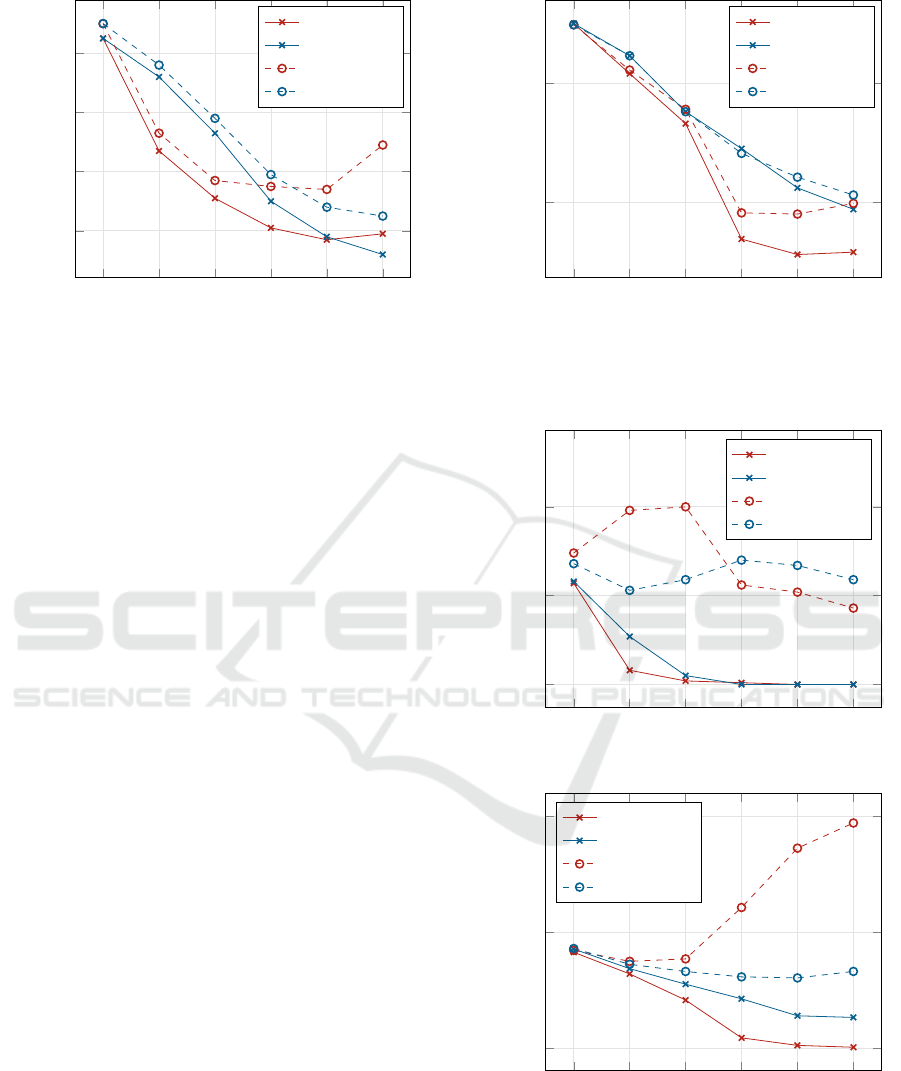
The losses after the 100 epochs for the training set
(T) and the validation set (V) are given in Fig. 3. The
KDIR 2023 - 15th International Conference on Knowledge Discovery and Information Retrieval
342

1 2 4 8 16 32
0.06
0.08
0.10
0.12
Number of convolutional layers
Loss
sequential T
parallel T
sequential V
parallel V
(a) MNIST.
1 2 4 8 16 32
1.70
1.80
Number of convolutional layers
Loss
sequential T
parallel T
sequential V
parallel V
(b) CIFAR10.
Figure 3: Sequential vs. parallel architecture: loss dependence on the number of residual convolutional layers (with a single
filter per layer) for the two datasets MNIST (left) and CIFAR10 (right).
performance of both architectures can be observed by
the points on the red (sequential architecture) and blue
(parallel variant) points. The solid lines represent the
training loss and the dashed lines the validation loss.
Due to their identical layout and equal random ini-
tialization, training the two networks with one con-
volutional layer and one filter each resulted conse-
quently in equal loss values.
It can be observed that both architectures per-
form similarly, in particular for the largest depths of
16 and 32. For MNIST, the shallow, parallel archi-
tecture slightly outperforms the original, sequential
one, while the relationship is inverse for the CIFAR10
dataset.
4.2 With Multiple Filters
A single-filter architecture is the most transparent one
but it is scarcely used. It is mostly assumed that more
filters are necessary to reach the desired classification
performance. Therefore, experiments with multiple
(1 to 32) filters per convolutional layer are included.
Same as before, the results after training for 100
epochs are shown in Figs. 4a and 4b. They show
an interesting development for CIFAR10: the train-
ing loss decreases by raising the number of filters
while the validation loss largely increases for more
than four filters. The validation loss considerably de-
teriorates for the sequential architecture. (The results
for MNIST are similar for the training set but less in-
terpretable for the validation set.)
The reason for the distinct picture on CIFAR10
is to be sought in relationships between constraints
imposed by the task and the number of free train-
able parameters (Hrycej et al., 2023, Chapter 4). A
task with K = 50,000 training examples constitutes
1 2 4 8 16 32
0.00
0.05
0.10
Number of Filters
Loss
sequential T
parallel T
sequential V
parallel V
(a) MNIST.
1 2 4 8 16 32
0.00
2.00
4.00
Number of Filters
Loss
sequential T
parallel T
sequential V
parallel V
(b) CIFAR10.
Figure 4: Sequential vs. parallel architecture: loss depen-
dence on the number of filters (with 16 convolutional lay-
ers) for the two datasets MNIST (left) and CIFAR10 (right).
Make Deep Networks Shallow Again
343

Table 1: Overdetermination ratios for both datasets and dif-
ferent model sizes based on the number of filters per convo-
lutional layer.
Overdetermination ratio Q
#filters #parameters MNIST CIFAR10
1 14k 41.771 34.804
2 37k 16.256 13.545
4 106k 5.630 4.691
8 344k 1.743 1.453
16 1.2M 0.495 0.412
32 4.5M 0.132 0.110
equally many constraints (resulting from the goal to
accurately match the target values) for each output
value. For 10 classes, there are M = 10 such output
values whose reference values are to be correctly pre-
dicted by the classifier. This creates KM constraints
(here: 50,000 × 10 = 500,000). For the mapping rep-
resented by the network, there are P free (i.e., mu-
tually independent) parameters to make the mapping
satisfy the constraints.
• With P = KM, the system is perfectly determined
and could be solved exactly.
• With P > KM, the system is underdetermined. A
part of the parameters is set to arbitrary values
so that novel examples from the validation set re-
ceive arbitrary predictions.
• With P < KM, the system is overdetermined, and
not all constraints can be satisfied. This may be
useful if the data are noisy, as it is not desirable to
fit to noise.
An appropriate characteristic is the overdetermination
ratio Q from (Hrycej et al., 2022) defined as
Q =
KM
P
(11)
The number of genuinely free parameters is difficult
to figure out. It can only be approximated by the total
number of parameters, keeping in mind that the num-
ber of actually free parameters can be lower.
In training a model by fitting to data, the presence
of the noise has to be considered. The model should
reflect the underlying genuine laws in the data but not
the noise. Fitting to the latter is undesirable and is the
substance of the well-known phenomenon of overfit-
ting. It was shown in (Hrycej et al., 2023, Chapter 4)
that fitting to the additive noise and thus the influence
of training set noise to the model prediction is reduced
to the fraction
1
/Q. In other words, it is useful to keep
the overdetermination ratio Q significantly over 1.
This supplementary information for the plotted
variants is given in Table 1. Acceptable values of the
overdetermination ratio Q are given with filter counts
of 1, 2, and 4. This is consistent with the finding that
overfitting did not take place in single-filter architec-
tures presented in Section 4.1.
For 8 filters or more, Q is close to 1 or even below
it. In this group, the validation loss can grow arbi-
trarily although the training loss is reduced. This is
the result of arbitrarily assigned values of underdeter-
mined parameters.
Altogether, the parallel architecture shows better
performance on the validation set despite the slightly
inferior loss on the training set. This can be attributed
rather to the random effects of underdetermined pa-
rameters than to the superiority of one or other ar-
chitecture. In this sense, both architectures can be
viewed as approximately equivalent concerning their
representational capacity.
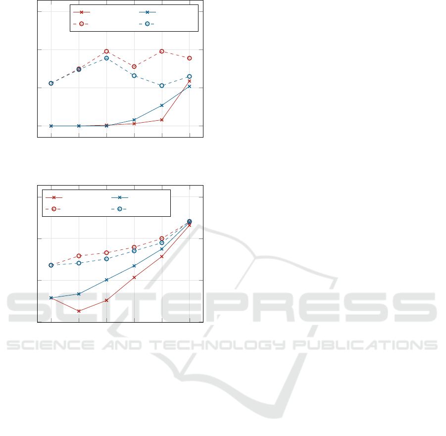
4.3 Trade-Off of the Number of Filters
and the Number of Layers
As an additional view to the relationship between the
depth and the width of the network, a group of exper-
iments is analyzed in which the product of the num-
ber of filters (F) and the number of convolution layers
(C) are kept constant. In this way, also “intermediary”
architectures between deep and shallow ones are cap-
tured. For example, an architecture with 32 filters and
a single convolutional layer has a ratio of
1
/32 while
the ratio with one filter and 32 layers is
32
/1. For 16
layers with each 8 filters, it is
16
/8 = 2.
For the product of 32, there are the following com-
binations of C × F: 1× 32, 2× 16, 4× 8, 8× 4, 16× 2
and 32 × 1. In Fig. 5, they are ordered along their
depth-width ratio
C
/F:
1
/32,
2
/16,
4
/8,
8
/4,
16
/2, and
32
/1.
These architectures are represented by the red curves.
As a reference, the blue curve shows their shallow
counterparts. Those are all single-layer architectures.
They differ only in the number of parameters, consis-
tent with their sequential counterparts represented by
the red curve. The difference in the number of pa-
rameters is due to the different sizes of the classifica-
tion layer following the residual connection sequence.
This classification layer is broader for more filters as
its input is larger the more filters there are.
Both the training and validation losses increase
with the depth-width ratio, indicating the superiority
of the shallow architectures. However, it is important
to note that this comparison may not be completely
fair due to the inherent difference in parameter num-
bers. Specifically, variants with higher depth-width
ratios have a diminishing number of parameters re-
sulting from their smaller number of filters.
In Figs. 5a and 5b, it can be observed that the
training loss for flattened alternatives is slightly larger
compared to the other architectures. However, the
KDIR 2023 - 15th International Conference on Knowledge Discovery and Information Retrieval
344

1
/32
2
/16
4
/8
8
/4
16
/2
32
/1
0.00
0.05
0.10
0.15
#layers
/#filters
Loss
sequential T parallel T
sequential V parallel V
(a) MNIST.
1
/32
2
/16
4
/8
8
/4
16
/2
32
/1
0.50
1.00
1.50
2.00
#layers
/#filters
Loss
sequential T parallel T
sequential V parallel V
(b) CIFAR10.
Figure 5: Sequential vs. parallel architecture: loss depen-
dence on the ratio of the numbers of layers and filters (prod-
uct of the number of layers and the number of filters is
fixed at 32) for the two datasets MNIST (left) and CIFAR10
(right).
validation loss for flattened alternatives is smaller, al-
beit to a moderate extent.
In summary, the deep variants can certainly not be
viewed as superior in overall terms. Both architec-
tures are roughly equivalent, as long as the number of
parameters is equal.
5 STATISTICS OF EXPERIMENTS
In addition to experiment runs selected for the presen-
tation in the previous sections, statistics over all 6,912
runs, partitioned into some categories, may be useful
to complete the performance picture. Of course, aver-
aging hundreds to thousands of experiments does not
guarantee to reflect all theoretical expectations suc-
cinctly; it can only confirm rough trends.
This statistical summary is presented in Table 2.
The losses for training and validation as well as for se-
quential and parallel architectures are partitioned into
intervals of overdetermination ratio to show the dif-
ferent behavior.
According to the theory, with a growing overde-
termination ratio, the discrepancy between training
and validation loss becomes smaller. On the other
hand, larger overdetermination ratios imply smaller
numbers of free network parameters. Sometimes, this
leads to increased losses from the diminished repre-
sentation capacity of the network. For ratios smaller
than 1, the validation loss may arbitrarily grow be-
cause of underdetermined parameters fitted to training
data noise (overfitting). This arbitrary growth may be
more or less articulated, depending mostly on random
factors. However, there is always a considerable risk
of such poor generalization.
As observed in the individual experiments pre-
sented, small discrepancies between training and val-
idation loss are reached for overdetermination ratios
larger than 3 for CIFAR10 and larger than 10 for
MNIST. These small discrepancies testify to good
generalization capability, expected for large overde-
termination ratios.
With Q < 1, the validation loss deteriorates for
CIFAR10 data if compared with the Q of the higher
interval. This is the effect of arbitrary parameter val-
ues caused by underdetermination.
To summarize, there is a slight advance of shallow
architectures for the validation set (five out of eight
categories), and deep architectures are better on the
training set. The training and validation losses are
mostly closer together for the parallel architecture.
6 CONCLUSION
It is stated in Section 2 that a deep residual connection
network can be approximately expanded into a sum of
shorter (i.e., less deep) sequences of different orders.
Truncating the expansion to the first two terms results
in a shallow architecture with a single layer. This sug-
gests a hypothesis that the representational capacity of
such a shallow architecture may be roughly as large as
that of the original deep architecture. If validated, this
hypothesis could open avenues to bypass issues typi-
cally associated with deep architectures.
Subsequent computational experiments conducted
on two widely recognized image classification tasks,
MNIST and CIFAR10, seem to confirm this theoret-
ically founded expectation. The performance of both
architectures (in configurations with identical num-
Make Deep Networks Shallow Again
345

Table 2: Mean training and validation loss for sequential and parallel architectures and various determination ratios Q inter-
vals.
Q ∈ [0, 1) Q ∈ [1,3) Q ∈ [3, 10) Q ∈ [10, ∞)
train val train val train val train val
MNIST
sequential 0.00013 0.05201 0.01702 0.12449 0.03620 0.11743 0.11246 0.13550
parallel 0.00009 0.07551 0.02679 0.11468 0.05238 0.11467 0.13310 0.14900
CIFAR10
sequential 0.25326 2.03107 0.72510 1.31691 1.07333 1.34721 1.58608 1.65354
parallel 0.52658 1.32386 0.88701 1.24884 1.17085 1.34227 1.63449 1.68879
bers of network parameters) is close to each other,
with a slight advance of shallow architectures in terms
of loss on the validation set.
While the deep architecture performed marginally
better on the training set, the cause of its underperfor-
mance on the validation set remains an open question.
It is plausible that the deep architecture’s ability to
capture abrupt nonlinearities may also make it prone
to overfitting to noise. In contrast, the shallow net-
work, due to its inherent smoothness, might exhibit a
higher tolerance towards training set noise.
In conclusion, our results suggest a potential par-
ity in the performance of deep and shallow architec-
tures. It is important to note that the optimization
algorithm utilized in this study is a first-order one,
which lacks guaranteed convergence properties. Fu-
ture research could explore the application of more ro-
bust second-order algorithms, which, while not com-
monly implemented in prevalent software packages,
could yield more pronounced results. This work
serves as a preliminary step towards reevaluating ar-
chitectural decisions in the field of neural networks,
urging further exploration into the comparative effi-
cacy of shallow and deep architectures.
REFERENCES
Fukushima, K. (1980). Neocognitron: A self-organizing
neural network model for a mechanism of pattern
recognition unaffected by shift in position. Biologi-
cal Cybernetics, 36(4):193–202.
He, K., Zhang, X., Ren, S., and Sun, J. (2016). Deep Resid-
ual Learning for Image Recognition. In 2016 IEEE
Conference on Computer Vision and Pattern Recog-
nition (CVPR), pages 770–778, Las Vegas, NV, USA.
IEEE.
Hinton, G. (2012). Neural Networks for Machine Learning.
Hrycej, T., Bermeitinger, B., Cetto, M., and Handschuh,
S. (2023). Mathematical Foundations of Data Sci-
ence. Texts in Computer Science. Springer Interna-
tional Publishing, Cham.
Hrycej, T., Bermeitinger, B., and Handschuh, S.
(2022). Number of Attention Heads vs. Number of
Transformer-encoders in Computer Vision. In Pro-
ceedings of the 14th International Joint Conference on
Knowledge Discovery, Knowledge Engineering and
Knowledge Management, pages 315–321, Valletta,
Malta. SCITEPRESS.
Krizhevsky, A. (2009). Learning Multiple Layers of Fea-
tures from Tiny Images. Dataset, University of
Toronto.
Krizhevsky, A., Sutskever, I., and Hinton, G. E. (2012). Im-
ageNet Classification with Deep Convolutional Neu-
ral Networks. In Advances in Neural Information Pro-
cessing Systems, volume 25. Curran Associates, Inc.
LeCun, Y., Boser, B., Denker, J. S., Henderson, D., Howard,
R. E., Hubbard, W., and Jackel, L. D. (1989). Back-
propagation Applied to Handwritten Zip Code Recog-
nition. Neural Computation, 1(4):541–551.
LeCun, Y., Bottou, L., Bengio, Y., and Haffner, P. (1998).
Gradient-based learning applied to document recogni-
tion. Proceedings of the IEEE, 86(11):2278–2324.
Meir, Y., Tevet, O., Tzach, Y., Hodassman, S., Gross, R. D.,
and Kanter, I. (2023). Efficient shallow learning as
an alternative to deep learning. Scientific Reports,
13(1):5423.
Mhaskar, H., Liao, Q., and Poggio, T. (2017). When and
Why Are Deep Networks Better Than Shallow Ones?
Proceedings of the AAAI Conference on Artificial In-
telligence, 31(1).
Russakovsky, O., Deng, J., Su, H., Krause, J., Satheesh, S.,
Ma, S., Huang, Z., Karpathy, A., Khosla, A., Bern-
stein, M., Berg, A. C., and Fei-Fei, L. (2015). Ima-
geNet Large Scale Visual Recognition Challenge. In-
ternational Journal of Computer Vision, 115(3):211–
252.
Simonyan, K. and Zisserman, A. (2015). Very Deep Con-
volutional Networks for Large-Scale Image Recogni-
tion.
Srivastava, R. K., Greff, K., and Schmidhuber, J. (2015).
Training very deep networks. In Advances in Neural
Information Processing Systems. Curran Associates,
Inc.
Tan, M. and Le, Q. (2019). EfficientNet: Rethinking model
scaling for convolutional neural networks. In Chaud-
huri, K. and Salakhutdinov, R., editors, Proceedings of
the 36th International Conference on Machine Learn-
ing, volume 97 of Proceedings of Machine Learning
Research, pages 6105–6114. PMLR.
KDIR 2023 - 15th International Conference on Knowledge Discovery and Information Retrieval
346