A Long-Term Funds Predictor Based on Deep Learning

Shuiyi Kuang and Yan Zhang

School of Computer Science and Engineering, California State University San Bernardino, U.S.A.

Keywords:

Fund Market Prediction, Gated Recurrent Units, Long Short-Term Memory, Deep Learning.

Abstract:

Numerous neural network models have been created to predict the rise or fall of stocks since deep learning has

gained popularity, and many of them have performed quite well. However, since the share market is hugely

inﬂuenced by various policy changes or unexpected news, it is challenging for investors to use such short-term

predictions as a guide. In this paper, a suitable long-term predictor for the funds market is proposed and tested

using different kinds of neural network models, including the Long Short-Term Memory (LSTM) model with

different layers, the Gated Recurrent Units (GRU) model with different layers, and the combination model

of LSTM and GRU. These models were evaluated on two funds datasets with various stock market technical

indicators added. Since the fund is a long-term investment, we attempted to predict the range of change in

the future 20 trading days. The experimental results demonstrated that the single GRU model performed best,

reached an accuracy of 92.14% to correctly predict the direction of rise or fall, and the accuracy of predicting

the speciﬁc change also hit 85.35%.

1 INTRODUCTION

With the rising inﬂation, it is necessary for many indi-

viduals and families to make some investments. The

greatest alternative among many investment options

is fund investment due to its convenience, low bar-

rier to entry, and low risk, especially for new investors

or those who are not familiar with the stock market.

The fund market predictor proposed in this paper is an

auxiliary application that helps fund investors decide

when to buy or sell stocks. Unlike a regular stock

market predictor, this predictor focuses more on the

fund market, which means that instead of targeting

a single stock, it largely targets a sector. It is more

likely to be correctly predicted because trends across

the industry are more stable than for a single stock.

In addition, the predictor takes some ﬁnancial mar-

ket indicators as input feature values, such as Raw

Stochastic Value (RSV), Standard Deviation (SD) and

Accumulation and Distribution Line (ACD). By train-

ing these data with ﬁnancial indicator features, an ef-

fective prediction model with the highest accuracy is

ﬁtted.

In this paper, Long Short-Term Memory (LSTM)

and Gated Recurrent Units (GRU), two variants of

the Recurrent Neural Network (RNN), are trained in

single-layer, multi-layer, and combined. The param-

https://orcid.org/0000-0002-5474-4019

eters such as the number of layers, number of neu-

rons, training period, single sample size, regulariza-

tion, dropout, and optimizer are adjusted by observing

the loss curve to obtain the optimal model.

Indeed, various prediction algorithms and models

have been proposed by many researchers in both aca-

demics and industry to predict the stock market ac-

curately. There have already been many successful

predictors for the stock market which can reach a rela-

tively high accuracy, but it is not that meaningful since

they could not help investors to make proﬁts in ac-

tual operations. People may know the stocks they are

holding will go down tomorrow but they do not know

the range of the price drop. What if you decide to sell

your shares but the price only drops a little, or you

decide to keep your shares but the price breaks down?

Warren Buffett, the most famous and successful in-

vestor, said it is unwise to decide one’s investment

whether failed or not only according to the next-day

stock price (Lowenstein, 2013). After all, investment

is a long-term business, especially for funds invest-

ment. It’s more important to keep track of the trends

rather than the ups and downs every day.

From a professional ﬁnancial point of view, even

if the fund market is more stable than the stock mar-

ket, the future is still uncertain. Policy shifts, bad

news from industry leaders, or the sudden outbreak

of war can cause unpredictable effects, so the predic-

Kuang, S. and Zhang, Y.

A Long-Term Funds Predictor Based on Deep Learning.

DOI: 10.5220/0012206400003598

In Proceedings of the 15th International Joint Conference on Knowledge Discovery, Knowledge Engineering and Knowledge Management (IC3K 2023) - Volume 1: KDIR, pages 347-354

ISBN: 978-989-758-671-2; ISSN: 2184-3228

347

tor is just an aid. As the old saying goes, you can

learn from history, and those who forget the past will

eventually repeat it. So, the signiﬁcance of the fund

predictor studied in this paper is to tell us not to make

similar unwise decisions that have been made many

times in history. Therefore, as ordinary investors who

do not have professional ﬁnancial knowledge, while

we choose an excellent fund, the speciﬁc manipu-

lation work will be done by professional fund man-

agers. All we need to do is deciding when to buy or

sell the shares. At this time, the fund predictor can

become a good assistant who offers supporting refer-

ence for you.

2 RELATED WORK

A review of the existing methods for the prediction of

the stock market using neural networks is discussed

in this section.

Cao et al. applied artiﬁcial neural networks to pre-

dict the stock price movements of companies traded

on the Shanghai Stock Exchange (Cao et al., 2005).

It is concluded that the neural network outperforms

the linear model and neural networks are useful tools

for stock price forecasting in emerging markets like

China. Yildiz et al. brought up a three-layer arti-

ﬁcial neural network to predict the rise and fall of

the ISE National-100 and achieved an accuracy of

74.51% (Yildiz et al., 2008). Hsieh et al. pro-

posed a Recurrent Neural Network (RNN) based on

the Artiﬁcial Bee Colony (ABC) algorithm to fore-

cast ﬁve indices including the Dow Jones Industri-

als (Hsieh et al., 2011). But the prediction was rel-

atively mediocre for time series data, since the RNN

network could not solve the problem of long-term

dependence. Nelson et al. examined the perfor-

mances of several different Long Short-Term Mem-

ory (LSTM) models, and got an average accuracy

of 55.9% in the ﬁnancial projection that whether a

single stock will rise in the coming period (Nelson

et al., 2017). The poor performance should prob-

ably be caused by the small amount of data and

the large variability of a single stock. Moghar and

Hamiche presented a 4-layer LSTM to predict NYSE

and GOOGLE and concluded that the prediction ac-

curacy increases with increasing epochs (Moghar and

Hamiche, 2020). Shao et al. applied the K-means

algorithm to cluster the stock price subseries (Shao

et al., 2017). An LSTM neural network model was

then constructed based on the number of clusters, and

the clustering results were used to train the corre-

sponding LSTM model, which resulted in higher pre-

diction accuracy than a single LSTM neural network

prediction model.

Gao et al. combined Long Short-Term Memory

(LSTM) and Gated Recurrent Units (GRU) for stock

market prediction and applied PCA and LASSO di-

mensionality reduction to the training data, and ﬁ-

nally concluded that LSTM and GRU have com-

parable predictive power, but LASSO dimensional-

ity reduction is more effective (Gao et al., 2021).

Roodiwala et al. developed a new LSTM model

which tracked the NIFTY 20 index for a period of 5

years, and ﬁnally achieved a Root Mean Square Er-

ror (RMSE) of merely 0.008, which was an excel-

lent performance (Roondiwala et al., 2017). Liu et

al. described a combination of a regularized GRU and

LSTM model, which yielded better results than either

GRU or LSTM alone (Liu et al., 2019). This novel

idea led us to consider the option of combining these

two neural networks for long-term prediction of fund

duration.

In these existing methods, the forecast targets are

short-term trends in highly volatile stocks, while we

choose to forecast long-term trends in more stable

funds, and to the exact range of the change, which

is more valuable for practical purposes.

3 DATASET

The source data used in this research was downloaded

from https://ﬁnance.yahoo.com/quote. We choose

two indices which track the ﬁnancial and real es-

tate sectors, respectively, for the period from January

2009 to November 2022. The ﬁnancial codes are

000934.SS and 000006.SS. After removing samples

with missing values, the total valid sample size ob-

tained was 3375, and the initial data contained 10 at-

tributes, as shown in Table 1.

Data from the ﬁnancial sector index is used to train

the model, and then data from the real estate sector

index is used to validate the model.

3.1 Financial Index Features

We add some ﬁnancial indicators to the original

dataset, and then manually extract features by calcu-

lating the correlation between the indicators. The in-

dicators with high correlations are dropped to reduce

the dimensions of input data, which can also increase

efﬁciency of neural network models.

The technical indicators commonly used in the ﬁ-

nancial markets (Kim, 2004) are added in the dataset,

as shown in Table 2.

As too many ﬁnancial indicators are added, the

dimension of the input becomes large,. The high-

KDIR 2023 - 15th International Conference on Knowledge Discovery and Information Retrieval

348

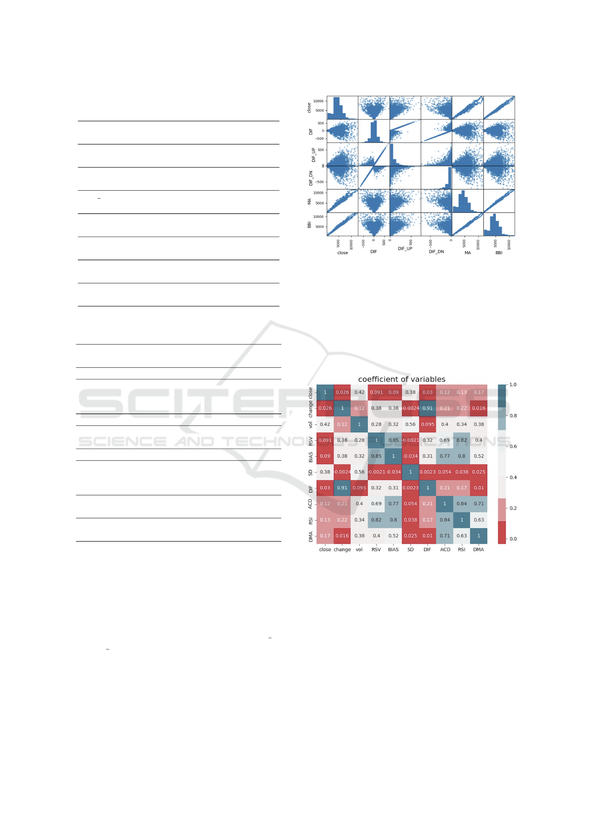
Table 1: Features and descriptions.

Features Description

Close The closing price at the end of the

day.

High The highest transaction price during

the whole day.

Low The lowest transaction price during

the whole day.

Pre close The closing price at the end of yes-

terday.

Range The price difference between today

and yesterday.

Change Percentage of the price difference

between today and yesterday.

Vol The number of shares traded in the

whole day.

Turnover A measure of the number of times

inventory is sold or used.

Table 2: Commonly used ﬁnancial index.

Feature Description

RSV Raw Stochastic Value, the most basic

stochastic value for each period.

MA Moving average of n-day price.

BIAS It reﬂects the deviation between the

price and its moving average in a cer-

tain period.

SD Standard Deviation of the price.

ACD Accumulation and Distribution Line,

it delivers buy and sell signals.

DIF Assistant indicator to calculate ACD.

RSI Relative Strength Index, a price fol-

lowing an oscillator which ranges

from 0 to 100.

DMA A security’s average closing price

over the previous 50 days.

BBI It measures the general short/mid-

term trend.

dimensional input is not conducive to the convergence

of the model. Therefore, we use a scatter plot to

show the indicators that are correlated computation-

ally, some indicators with strong linear correlation

can be found, and then those indicators can be elimi-

nated to reduce dimension.

Figure 1 shows that both MA and BBI are fully

positively correlated with the closing price, DIF UP

and DIF DN, which are intermediary products of DIF

calculation, are also positively correlated with DIF to

a large extent, so they can be deleted.

We generate the correlation coefﬁcient matrix by

calculating the correlation coefﬁcient between vari-

ables and show it by heat map in Figure 2. There is

Figure 1: Scatter graph of close, DIF, MA, and BBI.

a greater correlation between the variables when the

coefﬁcient of correlation is near 1. As shown in Fig-

ure 2, the blue parts can be considered a very high

correlation, so they can be eliminated. Besides, RSV,

BIAS, DMA, RSI are relatively highly correlated, so

it’s enough to only keep RSV indicator. DIF indicator

also has a very strong correlation with daily change,

so it can be eliminated as well.

Figure 2: Heat map of coefﬁcients of existing features.

Figure 3 shows the ﬁnal features of remained six

characteristic values of input data, including closing

price, up and down change, trading volume, RSV,

SD, and ACD, which have a relatively low correlation

with each other.

3.2 Trend of Index as Output

For a long-term fund investor, holding the fund for

more than one month is a basic strategy, so the pro-

posed model is designed to predict the future trend of

the fund within 20 trading days. The trend of the in-

A Long-Term Funds Predictor Based on Deep Learning

349

Figure 3: The extracted 6 features.

dex for the next 20 trading days will be used as the

forecast target. After streamlining the input data, a

new feature disparity 20 is added, which is the cu-

mulative increase or decrease over the next 20 trading

days. The latest 20 samples will be discarded because

it is impossible to calculate. Since the calculation of

RSV needs to use the lowest and highest prices of the

past 20 trading days, the oldest 20 samples will be

discarded because they cannot be calculated. Finally,

3335 samples out of 3375 original samples are in the

dataset. The six reﬁned indicators are used as input

data, while the future 20-day change disparity 20 is

used as output data.

3.3 Data Normalization and Split

To ensure robust model convergence and prevent ex-

tended training times caused by numerous eigenval-

ues with varying magnitudes and units, we employ a

variant of Min-Max normalization to scale the data

within the range of [−1, 1]. As a beneﬁt of normaliza-

tion, the training model is able to converge more eas-

ily since the data are in the same order of magnitude.

The preprocessed data are divided into a training set,

validation set, and test set by the ratio of 7 : 2 : 1.

4 METHODOLOGY

This experiment tests ﬁve models for long-term pre-

diction of funds markets to select the most suitable

one: single-layer LSTM, single-layer GRU, multi-

layer LSTM, multi-layer GRU, and hybrid GRU-

LSTM. RNN model is examined ﬁrst since the LSTM

and GRU models are frequently cited as suitable RNN

variations for time series forecasting.

4.1 RNN

Compared to standard neural networks, RNNs can

connect past information to current tasks, making

them valuable for solving time series prediction prob-

lems. (Medsker and Jain, 2001). The structure of

RNNs determines that it can only receive information

from the approaching moment when processing infor-

mation at the current moment. It cannot receive infor-

mation from an earlier moment. There is only one

activation function inside the standard RNN , usually

tanh or so f tsign.

RNNs retain the information of past moments in

the forward propagation process. When optimizing

the model, the gradient descent method is used to up-

date the parameter values along the direction of the

gradient of the objective function to achieve the min-

imum loss value. When the gradient approaches 0,

it signiﬁes negligible impact, a key challenge in us-

ing RNN for long time series problems. Thus, it also

gives birth to RNN variant forms, LSTM and GRU, to

solve the gradient disappearance.

4.2 LSTM

LSTM adds a cell state and three gate structures to

achieve the retention of information. Three gates

are the input gate, the forgetting gate, and the out-

put gate (Yu et al., 2019). The forgetting gate is the

key to the LSTM, and it determines what information

is forgotten and what information is added to the cell

state (Yu et al., 2019). The internal structure of the

LSTM is shown in Figure 4.

Figure 4: The internal structure of LSTM.

Initially, h

t−1

and x

pass through the forgetting

gate (typically a sigmoid function), yielding f

in the

range (0,1) where 1 retains all and 0 forgets all. Then,

the input gate computes i

via a sigmoid function, de-

termining what to retain and introducing new infor-

mation through a tanh function. Lastly, the updated

cell state, conﬁned to (−1, 1) by a tanh function, is

multiplied by the output gate result o

to produce the

KDIR 2023 - 15th International Conference on Knowledge Discovery and Information Retrieval

350

ﬁnal output h

. Thus, we only need to set a larger bias

term for the forgetting gate of LSTM, then the cell

state can maintain a relatively stable gradient ﬂow,

which can also alleviate the gradient disappearance

problem due to fractional concatenation.

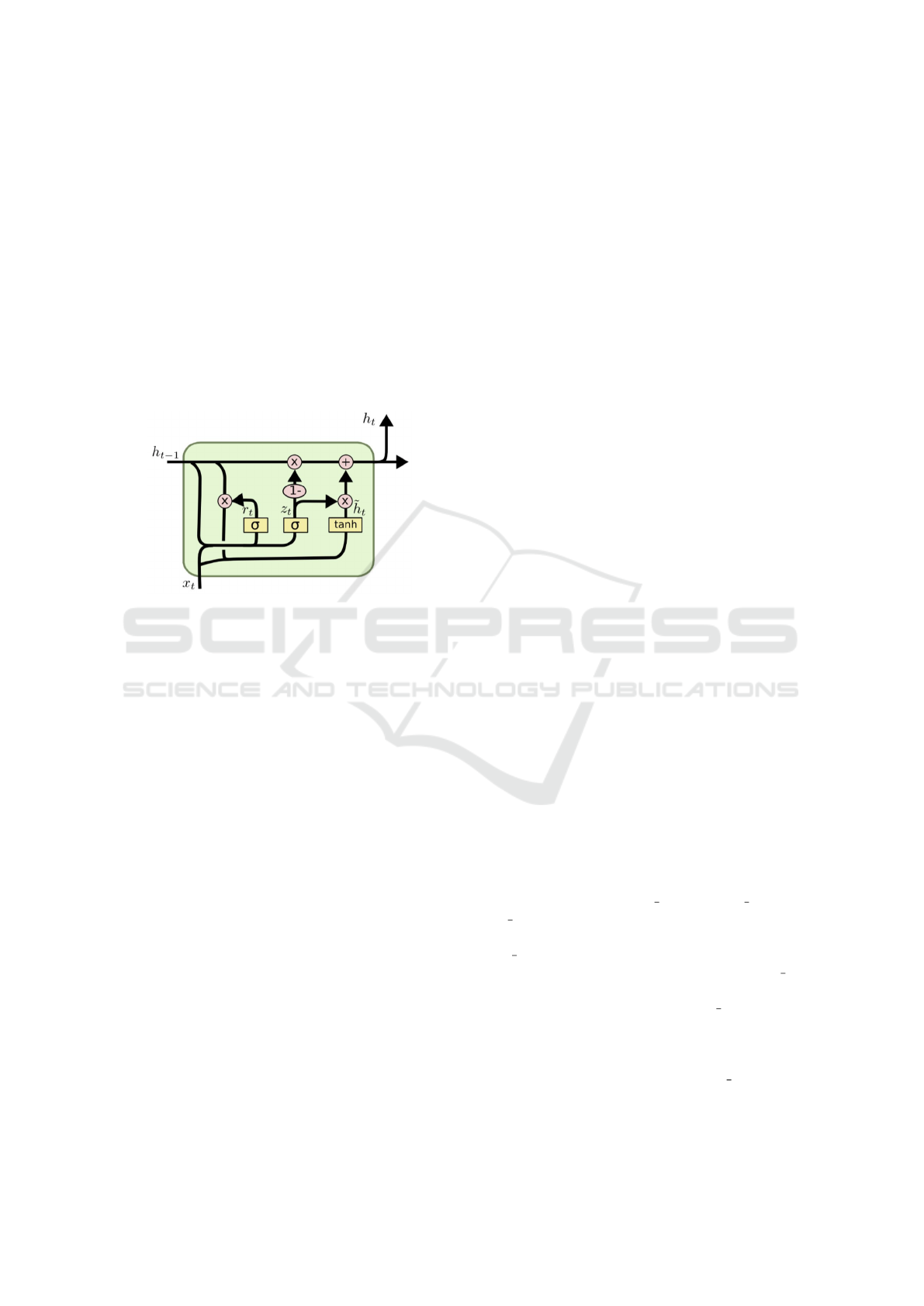
4.3 GRU

GRU, a concise version of LSTM, combines the for-

getting gate and input gate into one update gate and

merges cell state and hidden state, which greatly sim-

pliﬁes the structure of LSTM but achieves a similar

effect as LSTM (Chen et al., 2019). The internal

structure of GRU is shown in Figure 5.

Figure 5: The internal structure of GRU.

GRU only has two gates, a reset gate and an up-

date gate, which are computed in the same way as the

gates in LSTM. GRU has one less gate than LSTM, so

the total number of parameters is only three-quarters

of LSTM with same complexity. GRU is more con-

cise and reduces the risk of overﬁtting. It is also able

to deal with both long-term and short-term dependen-

cies.

4.4 Stacked Neural Network

Multi-layer neural network stacking is utilized to im-

prove the learning ability of a model, where multi-

ple hidden layers are added between the input and

the output layer, and the output of the former layer is

passed to the latter layer with the same dimension as

the input (Mohammadi and Das, 2016). Nevertheless,

given that stacking multi-layer neural networks can

cause issues related to gradient vanishing and overﬁt-

ting, this experiment primarily focuses on two-layer

stacked networks. There are an input layer, two mid-

dle layers and an output layer. The middle layers can

be RNN, LSTM, or GRU. This experiment will test

the stacked neural network in three ways: double-

layer LSTM, double-layer GRU, and mixed GRU-

LSTM.

4.5 Evaluation Methods

We use ﬁve evaluation criteria, namely Mean Abso-

lute Error (MAE), Root Mean Square Error (RMSE),

score, Probability, and Accuracy to evaluate the

prediction performance of the selected models.

The MAE is used to measure the mean absolute

error between the predicted and true values, which is

deﬁned as follows. A smaller MAE means a better

model (Hodson, 2022).

RMSE is used to indicate how much error the

model will produce in the prediction, similar to the

standard deviation. It allows for assessing the stabil-

ity of the model (Hodson, 2022).

is a default model evaluation metric used by

scikit-learn in the implementation of linear regres-

sion, which can be used to reﬂect the degree of the

model’s ﬁtness to the data. The larger it is, the better

the model is (Hodson, 2022).

Probability is the probability of correctly predict-

ing the rise and fall trend in all test samples. It is an

evaluation criterion especially set in this research.

Accuracy is an evaluation criterion especially set

in this paper. Since the purpose of this test is to predict

the future of the 20 trading days, this indicator is used

to show the probability that the difference between the

real changes and predicted changes is within 0.02 or

less. As long as the gap between predicted changes

and the actual changes is less than 0.02, it is consid-

ered as a valid prediction.

5 EXPERIMENTS AND RESULTS

5.1 Parameters Setting

LSTM and GRU have similar parameter conﬁgura-

tions, including input data shape, neural unit count,

batch size, epoch, loss, activation, optimizer, archi-

tecture, and reliability.

Data Shape: As LSTM and GRU expect three-

dimensional tensors (input length, input size, and

time step), the two-dimensional data should be re-

shaped into three-dimensional data in advance. The

input length is the length of the original data, and it

is the total number of 3335 samples. The input size

is the number of features of the extracted ﬁnancial in-

dicators after preprocessing. The time step is set to 1

for the single stock data, where the dimension of each

sample is 1, then the length of the data processed by

each time step is just 1. If we are dealing with two-

dimensional image data, then the time

step will in-

crease to the vertical length of the image.

A Long-Term Funds Predictor Based on Deep Learning

351

Neural Unit Count: The number of neural units im-

pacts both model parameters and output dimensional-

ity, which need to be adjusted according to the results

during the training process. Adjustments should align

with training results — increasing the number of units

if a model is underﬁtting and decreasing it when over-

ﬁtting.

Batch Size: Batch size determines the number of

samples processed per training step. The loss value

calculated in model optimization is the average loss

of all samples in a single batch size. A larger batch

size will lead to memory consumption, slow speed,

and inaccuracy problems. While a smaller batch size

may result in convergence difﬁculties. Therefore, it is

very important to choose a suitable batch size to im-

prove the running speed and increase the accuracy of

gradient descent.

Epoch: Epoch represents one complete dataset pass

through the network. We need to pass the complete

dataset in the same neural network several times to

keep updating the weight matrix of the network to

reach the optimal solution. However, multiple epochs

are essential with more potentially leading to overﬁt-

ting. The appropriate number depends on the training

process and requires adjustment. We set 10 epochs as

the monitoring period in this experiment.

Loss: All test models in this experiment use mean

average error as the loss value.

Activation Function: Activation functions determine

information retention. Due to the changes can be both

positive and negative, Tanh with the symmetric nor-

malization range as (-1,1) is chosen. Other suitable

activation functions will be tested to ensure the most

suitable one for the model.

Optimizer: The optimizer optimizes the weights and

bias parameters during gradient descent. The default

Adam optimizer is used. Alternative optimizers will

be tested to see how they work.

Model Architecture: The GRU-LSTM model in this

paper refers to the ﬁve-layer neural network model

proposed in (Liu et al., 2019), with the input and out-

put layers, two layers of GRU and one layer of LSTM

as hidden or middle layers. L2 regularization is used

to avoid the risk of overﬁtting with the increase in the

number of intermediate layers

Dropout: To avoid overﬁtting, dropout is applied

during training, which means temporarily deactivat-

ing neural units with a certain probability (Srivastava

et al., 2014). Since it is a temporary random dropout

for each batch-size sample in different networks, it

forces each neural unit to work together with other

randomly selected neural units, weakening the joint

adaptation between neurons. Thus, it achieves the ef-

fect of suppressing overﬁtting and enhancing general-

ization ability.

Reliability: Due to neural network variability, even if

using the same data to train the same model multiple

times, the obtained result in each run could be differ-

ent. To ensure the reliability of the training process,

each parameter adjustment is repeated 10 times, and

average validation set loss will be taken as the refer-

ence and depicted using box plots.

In the process of adjusting the parameters, every

time a parameter is changed, other parameters need

to be retested along with it. Thus, to improve the efﬁ-

ciency, the loss curve in the test process will be used

to determine whether it is in an overﬁtting or under-

ﬁtting state, and the test range of the parameters will

be adjusted accordingly. We use boxplots which is a

graphical representation of a distribution of numeri-

cal data, to show the variation of loss in response to

changes of one certain independent variable.

The ﬁnal parameters of each model are shown in

Table 3.

5.2 Results

This experiment uses the Keras neural network ar-

chitecture to build prediction models (Gulli and Pal,

2017). To compare the prediction performance,

for each model we train and predict on a fund

index dataset tracking the ﬁnancial sector (code

000934.SS), and then use the model with same pa-

rameters on another dataset tracking the real estate

sector (code 000006.SS). Each model is trained 20

times on each dataset and then the results are aver-

aged. The forecast results of the models for fund in-

dices 000934.SS and 000006.SS are shown in Table 4.

From Table 4, it is obvious that among all ﬁve

models for forecasting the two fund indices, the

single-layer GRU model performs the best, with the

lowest error and the highest model ﬁt. The stan-

dard deviation in the last column shows that the GRU

model performs the most consistently over the course

of 20 repeated trials, with an MAE standard deviation

for only 0.0002 over 20 trials. As for the most crucial

criterion Accuracy, the single-layer GRU model per-

forms signiﬁcantly more accurately than other mod-

els, reaching an accuracy rate of 85.35% in predicting

the change of the fund (000934.SS) with ﬂuctuations

within 2%. However, the same model is much less ef-

fective in predicting another fund (000006.SS), with

an accuracy of 71.40%, which may result from the

fact that the adjustment process of the model parame-

ters is based on a single data set.

The performances of the ﬁve models are compara-

ble when it comes to the effect of the up and down pre-

diction, all reaching about 90%. It is evident that just

KDIR 2023 - 15th International Conference on Knowledge Discovery and Information Retrieval

352

Table 3: The parameters of each model.

LSTM Stacked-LSTM GRU Stacked-GRU GRU+LSTM

1st-units 30 40 50 50 50

2nd-units − 50 − 20 20

3rd-units 3 − − − − 30

batch size 20 70 20 70 32

epoch 10 40 25 40 25

dropout 0.2 0.4 0.2 0.4 0.4

activation softsign softsign tanh softsign softsign

optimizer adam adam adam adam adam

Table 4: Experimental results.

Code Model MAE RMSE Rsquare Prob Acc Std(MAE)

000934.SS LSTM 0.0135 0.0173 0.8754 91.72% 76.63% 0.0005

GRU 0.0109 0.0142 0.9160 92.14% 85.35% 0.0002

Stacked-LSTM 0.0134 0.0169 0.8807 90.50% 78.80% 0.0008

Stacked-GRU 0.0153 0.0190 0.8495 89.89% 72.09% 0.0011

GRU-LSTM 0.0128 0.0163 0.8894 90.25% 79.23% 0.0009

000006.SS LSTM 0.0169 0.0222 0.8861 90.26% 67.94% 0.0006

GRU 0.0150 0.0206 0.9022 90.97% 71.74% 0.0050

Stacked-LSTM 0.0168 0.0219 0.8895 90.88% 66.93% 0.0005

Stacked-GRU 0.0181 0.0231 0.8775 89.94% 61.48% 0.0009

GRU-LSTM 0.0192 0.0242 0.8638 88.98% 59.91% 0.0026

simply predicting the up and down is relatively easy,

although it could not offer very meaningful guidance

to practical operation. However, if combined with the

prediction graph shown in Figure 6 and 7, it can be

seen that the failure to predict the direction of the rise

and fall is mainly concentrated in the areas near x-

axis, which means the range of change is very small.

For long-term fund investors, a such small change can

be ignored, which means that when the prediction re-

sults in small ﬂuctuations, the actual prediction accu-

racy rate will be higher than the average accuracy rate

of statistics.

Figure 6 and 7 show the prediction curve of the

best-performing GRU model for two fund indices.

The red line is the true value and the green line is

the predicted value. The closer they are, the better the

prediction is.

It is easy to see that the largest forecast errors tend

to occur at the time of the largest increases or de-

creases. Therefore, such recent forecast effect graphs

can be quite instructive when making an artiﬁcial

judgment of long-term trends.

6 CONCLUSIONS

In this research, ﬁve neural network models for pre-

dicting long-term fund trends were trained and tested

on two datasets 000934.SS and 000006.SS. We con-

Figure 6: Prediction curve of single GRU on 000934.SS.

cluded that the single-layer GRU model has the best

performance, with an effective prediction accuracy of

85.35% on dataset 000934.SS. Although the whole

process of adjusting the parameters is done based on

this dataset, which leads to a slightly worse predic-

tion effect of the same model on other datasets. The

effective prediction accuracy declined to 71.40% on

dataset 000006.SS. On the other hand, we can have

A Long-Term Funds Predictor Based on Deep Learning

353

Figure 7: Prediction curve of single GRU on 000006.SS.

reasons to believe that the prediction accuracy can

be greatly improved by making special model adjust-

ments for speciﬁc funds. The reliability of different

prediction results can also be determined by subjec-

tive judgment with the assistance of recent prediction

curves, so long-term prediction of fund trends through

deep learning is feasible.

The purpose of this experiment is to build an aux-

iliary forecaster through deep learning. After all, the

ﬁnancial market is hugely variable and greatly inﬂu-

enced by the news, so the role of deep learning is

more of a technical prediction. It can only be used

as a reference, but not as a decisive factor. Therefore,

a single-layer GRU neural network model with such

prediction accuracy is already a surprise and fully suf-

ﬁcient. In the future, the process of adjusting the pa-

rameters of neural networks can be streamlined and

made more efﬁcient. The AI-driven training meth-

ods can be adopted to simplify the task signiﬁcantly.

Continuing this research, our aim is to transform the

auxiliary predictor developed here into a versatile tool

that can beneﬁt a broader audience, facilitating invest-

ment decisions for a wide range of individuals.

REFERENCES

Cao, Q., Leggio, K. B., and Schniederjans, M. J. (2005).

A comparison between fama and french’s model and

artiﬁcial neural networks in predicting the chinese

stock market. Computers & Operations Research,

32(10):2499–2512.

Chen, J., Jing, H., Chang, Y., and Liu, Q. (2019). Gated

recurrent unit based recurrent neural network for re-

maining useful life prediction of nonlinear deteriora-

tion process. Reliability Engineering & System Safety,

185:372–382.

Gao, Y., Wang, R., and Zhou, E. (2021). Stock prediction

based on optimized lstm and gru models. Scientiﬁc

Programming, 2021:1–8.

Gulli, A. and Pal, S. (2017). Deep learning with Keras.

Packt Publishing Ltd.

Hodson, T. O. (2022). Root-mean-square error (rmse) or

mean absolute error (mae): When to use them or

not. Geoscientiﬁc Model Development, 15(14):5481–

5487.

Hsieh, T. J., Hsiao, H. F., and Yeh, W. C. (2011). Forecast-

ing stock markets using wavelet transforms and recur-

rent neural networks: An integrated system based on

artiﬁcial bee colony algorithm. Applied soft comput-

ing, 11(2):2510–2525.

Kim, K.-j. (2004). Toward global optimization of case-

based reasoning systems for ﬁnancial forecasting. Ap-

plied intelligence, 21:239–249.

Liu, Y. W., Wang, Z. P., and Zheng, B. Y. (2019). Appli-

cation of regularized gru-lstm model in stock price

prediction. In 2019 IEEE 5th International Con-

ference on Computer and Communications (ICCC),

pages 1886–1890. IEEE.

Lowenstein, R. (2013). Buffett: The making of an American

capitalist. Random House.

Medsker, L. R. and Jain, L. (2001). Recurrent neural net-

works. Design and Applications, 5(64-67):2.

Moghar, A. and Hamiche, M. (2020). Stock market pre-

diction using lstm recurrent neural network. Procedia

Computer Science, 170:1168–1173.

Mohammadi, M. and Das, S. (2016). Snn: stacked neural

networks. arXiv preprint arXiv:1605.08512.

Nelson, D. M. Q., Pereira, A. C. M., and De Oliveira, R. A.

(2017). Stock market’s price movement prediction

with lstm neural networks. In 2017 International joint

conference on neural networks (IJCNN), pages 1419–

1426. IEEE.

Roondiwala, M., Patel, H., and Varma, S. (2017). Predict-

ing stock prices using lstm. International Journal of

Science and Research (IJSR), 6(4):1754–1756.

Shao, X. L., Ma, D., Liu, Y. W., and Yin, Q. (2017). Short-

term forecast of stock price of multi-branch lstm based

on k-means. In 2017 4th International Conference on

Systems and Informatics (ICSAI), pages 1546–1551.

IEEE.

Srivastava, N., Hinton, G., Krizhevsky, A., Sutskever, I.,

and Salakhutdinov, R. (2014). Dropout: a simple way

to prevent neural networks from overﬁtting. The Jour-

nal of Machine Learning Research, 15(1):1929–1958.

Yildiz, B., Yalama, A., and Coskun, M. (2008). Forecasting

the istanbul stock exchange national 100 index using

an artiﬁcial neural network. An International Journal

of Science, Engineering and Technology, 46:36–39.

Yu, Y., Si, X. S., Hu, C. H., and Zhang, J. X. (2019). A re-

view of recurrent neural networks: Lstm cells and net-

work architectures. Neural computation, 31(7):1235–

1270.

KDIR 2023 - 15th International Conference on Knowledge Discovery and Information Retrieval

354