Evaluating the Use of Interpretable Quantized Convolutional Neural

Networks for Resource-Constrained Deployment

Harry Rogers

1 a

, Beatriz De La Iglesia

1 b

and Tahmina Zebin

2 c

School of Computing Science, University of East Anglia, U.K.

School of Computer Science, Brunel University London, U.K.

Keywords:

Class Activation Maps, Deep Learning, Quantization, XAI.

Abstract:

The deployment of Neural Networks on resource-constrained devices for object classiﬁcation and detection

has led to the adoption of network compression methods, such as Quantization. However, the interpretation

and comparison of Quantized Neural Networks with their Non-Quantized counterparts remains inadequately

explored. To bridge this gap, we propose a novel Quantization Aware eXplainable Artiﬁcial Intelligence (XAI)

pipeline to effectively compare Quantized and Non-Quantized Convolutional Neural Networks (CNNs). Our

pipeline leverages Class Activation Maps (CAMs) to identify differences in activation patterns between Quan-

tized and Non-Quantized. Through the application of Root Mean Squared Error, a subset from the top 5%

scoring Quantized and Non-Quantized CAMs is generated, highlighting regions of dissimilarity for further

analysis. We conduct a comprehensive comparison of activations from both Quantized and Non-Quantized

CNNs, using Entropy, Standard Deviation, Sparsity metrics, and activation histograms. The ImageNet dataset

is utilized for network evaluation, with CAM effectiveness assessed through Deletion, Insertion, and Weakly

Supervised Object Localization (WSOL). Our ﬁndings demonstrate that Quantized CNNs exhibit higher per-

formance in WSOL and show promising potential for real-time deployment on resource-constrained devices.

1 INTRODUCTION

As technology progresses, the ﬁeld of Artiﬁcial In-

telligence (AI) continues to advance enabling more

sophisticated solutions. Typically, for automated

image-processing tasks, Vision Transformers (ViTs)

and variants of deep Convolutional Neural Networks

(CNNs) are commonly employed for object classiﬁ-

cation and detection. However, as researchers pro-

pose increasingly complex architectures, these archi-

tectures are becoming larger and more computation-

ally intensive, posing challenges for training and in-

ference time. Moreover, the hardware limitations of

resource-constrained devices further complicate the

deployment of these larger networks. As a result, re-

searchers have turned to compression methodologies

to address these challenges.

To tackle the need for efﬁcient model deploy-

ment and inference on devices with limited resources,

quantization has emerged as a promising technique.

https://orcid.org/0000-0003-3227-5677

https://orcid.org/0000-0003-2675-5826

https://orcid.org/0000-0003-0437-0570

By reducing the memory footprint and computational

requirements of Neural Networks, Quantized net-

works offer a viable solution that balances model size

and inference speed while maintaining acceptable lev-

els of accuracy.

Quantization involves converting Neural Network

weights from 32-bit ﬂoating-point to 8-bit integer rep-

resentation, reducing memory usage and computa-

tion requirements without sacriﬁcing accuracy. By

leveraging the beneﬁts of quantization, larger and

more complex models can be deployed on resource-

constrained devices. The reduced memory footprint

and faster inference time make Quantized CNNs par-

ticularly suitable for real-time applications

In this paper, we explore the application of quanti-

zation on CNNs, aiming to leverage the beneﬁts of re-

duced memory usage and faster inference times using

publicly available architectures from PyTorch (Paszke

et al., 2019). We investigate the impact of quan-

tization on CNN activations, CNN accuracy, CNN

size, and inference speed. Our goal is to provide

insights into the trade-offs and advantages of Quan-

tized networks for efﬁcient deployment on resource-

constrained devices in a Weakly Supervised Object

Rogers, H., De La Iglesia, B. and Zebin, T.

Evaluating the Use of Interpretable Quantized Convolutional Neural Networks for Resource-Constrained Deployment.

DOI: 10.5220/0012231900003598

In Proceedings of the 15th International Joint Conference on Knowledge Discovery, Knowledge Engineering and Knowledge Management (IC3K 2023) - Volume 1: KDIR, pages 109-120

ISBN: 978-989-758-671-2; ISSN: 2184-3228

109

Localization (WSOL) task.

Within literature, there has not been a comparison

drawn between Quantized and Non-Quantized CNNs

to identify regions of interest. Proposed in this pa-

per is an Quantization Aware eXplainable AI (XAI)

pipeline to visualize and compare regions of interest

between Quantized and Non-Quantized CNNs using

Class Activation Maps (CAMs). CAMs are computed

using the last convolutional layer in a speciﬁed CNN.

In this paper we use EigenCAM (Bany Muhammad

and Yeasin, 2021) as the method for CAM compu-

tation is gradient-free, allowing for activation only

inference. Using CAMs from Quantized and Non-

Quantized CNNs, Root Mean Squared Error (RMSE)

is applied to identify differences between CAMs. Af-

ter taking the top 5% where the CAMs are different,

we create a subset of images to test. Using this sub-

set, we apply several metrics to activations to identify

differences between Quantized and Non-Quantized

CNNs. To evaluate CAM effectiveness XAI metrics

Deletion and Insertion are applied with a WSOL task.

To facilitate the contrast between networks we use the

ImageNet dataset (Russakovsky et al., 2015). Our

usage of WSOL is intended to allow for resource-

constrained devices to have a lightweight object de-

tector on board without the need for training a more

complex model that cannot be deployed due to its

size.

The core contributions of this paper are as follows:

1. Comparison of Quantized CNNs and Non-

Quantized CNNs using XAI to identify different

regions and features utilized for image classiﬁca-

tion.

2. Comparison of Quantized CNNs and Non-

Quantized CNNs in a Weakly Supervised Object

Localization task, considering the feasibility in

real-time usage.

3. Comparison of Quantized and Non-Quantized ac-

tivation blocks using several statistical metrics, to

identify similarities and differences.

The remainder of the paper is organized as follows.

Section 2 presents related literature on quantization

methods, with a focus on the application of XAI

methods. It also provides a review of XAI CAM

methods and their evaluations. Section 3 presents the

details of the Quantization Aware XAI pipeline, in-

cluding CAM evaluation metrics, activation metrics,

classiﬁcation metrics, inference speed test informa-

tion, and ImageNet baselines with the applied quanti-

zation methodologies. The performance of CAM ex-

planations is reported and evaluated in Section 4. Fi-

nally, Section 5 presents the conclusions of the paper

and outlines future work.

2 RELATED LITERATURE

Quantized Neural Networks have been combined with

XAI with differing methodologies to enable more ef-

ﬁcient deployment and use of Neural Networks. The

combination of CAMs and Quantized Neural Net-

works has been identiﬁed in literature but not fully

explored as we do in this paper.

2.1 Quantization and Explainable

Quantization

Quantization was originally proposed to be used for

faster inference times for mobile devices with real-

time deployment. Jacob et al. (2017) was the ﬁrst to

propose Quantization Aware Training (QAT) which

involves training Neural Networks directly with low-

bit Quantized weights and activations. QAT maintains

the performance of higher bit Non-Quantized weights

and activations whilst achieving inference speed-ups

as well as a lower memory usage. Quantization is

achieved through the usage of straight-through esti-

mation. The method approximates gradients during

backpropagration to account for the reduction of in-

formation from quantization, converting 32-bit ﬂoat-

ing point values into lower bit values.

Following that, there have been many methodolo-

gies to achieve a more efﬁcient inference using quan-

tization with the aim of minimising the error from

quantization (Gholami et al., 2021; Ghimire et al.,

2022; Liang et al., 2021). Various optimization meth-

ods have been explored to enhance the performance of

Neural Networks on hardware with limited computa-

tional power. These methods include hardware-aware

training, which aims to improve network efﬁciency

on speciﬁc hardware platforms. Additionally, zero-

shot quantization techniques have been employed to

convert weights and activations without the need for

retraining or ﬁne-tuning, similar to post static quan-

tization. These approaches collectively contribute to

improving Neural Network efﬁciency and adaptabil-

ity on resource-constrained hardware. However, each

method may be good on a speciﬁc test case, but may

have downsides when compared to each other; there

seems too not be a universal best ﬁt.

Since the adoption of Quantized networks, devel-

opments have been made to make networks more ef-

ﬁcient with other compression methods. For exam-

ple, pruning by removing weights has been used in

conjunction with quantization (Xu et al., 2020; Liu

et al., 2020). Pruning methods can be structured or

unstructured, where structured refers to removing en-

tire nodes from a network and unstructured refers to

setting speciﬁc parameters to zero, making the net-

KDIR 2023 - 15th International Conference on Knowledge Discovery and Information Retrieval

110

work sparse. Both methods make networks lighter

and can have speed-ups whilst retaining accuracy.

Pruning has been used with Quantized networks and

XAI with the usage of Deep Learning Important Fea-

Tures (DeepLIFT) (Shrikumar et al., 2019) to make

models lighter and more efﬁcient (Sabih et al., 2020).

DeepLIFT operates by assigning importance scores to

individual input features based on the difference they

make in the networks activations compared to a refer-

ence baseline. The usage of XAI is an excellent way

to identify weights in a network that could be pruned

as they serve no purpose for inference. However,

Sabih et al. (2020) could have a comparison to the

Non-Quantized counterpart to show key differences to

highlight improvements. Furthermore, usage of other

XAI methods following this should be explored.

Methods such as guided backpropogation with

Quantized networks have been explored in the liter-

ature. For example, Zee et al. (2022) compares a

Quantized CNN to a Non-Quantized baseline CNN,

pruned CNN, ablated CNN, and a pruned and Quan-

tized CNN. The usage of guided backpropogation re-

sults in a CAM for each CNN, however, there are no

metrics used to evaluate the CAMs with regards to

how effective each CAM is at representing what the

CNN actually uses for prediction. Furthermore, there

is only one Quantized CNN tested with QAT.

Similar research has been completed with image

retrieval tasks with explainable Quantized CNNs (Ma

et al., 2023). A novel quantization methodology,

Deep Progressive Asymmetric Quantization, is pro-

posed and CNNs are visualised with CAMs. The

CAM method utilised is not evaluated with metrics

like Zee et al. (2022). There also is no comparison to

a Non-Quantized CNN counterpart to identify what

baselines could be achieved.

From our review of quantization, it can be stated

there are many methodologies for quantization but not

all are openly available online. A key part of research

is being able to replicate results and data, therefore

for this paper we will use pretrained weights that are

publicly available from PyTorch. Comparing quanti-

zation methods to the Non-Quantized counterpart has

also not been fully explored, with little research on

publicly available datasets. Therefore, comparisons

between QAT and Post Static quantization of CNNs

using the ImageNet dataset will be explored in this

paper.

2.2 Class Activation Maps and

Evaluations

Within XAI there are methods to identify regions

of interest from CNN predictions. These methods

visualise gradients or activations from CNN predic-

tions by taking the last layer of the architecture and

computing regions of interest called Class Activation

Maps (CAMs). Previously, gradient based methods

have been used with GradCAM, GradCAM++, Full-

Grad, with success (Selvaraju et al., 2019; Chattopad-

hay et al., 2018; Srinivas and Fleuret, 2019). More

recently, gradient-free methodologies have been used

to account for networks that can have negative or non-

differentiable values within gradients.

AblationCAM was one of the ﬁrst gradient-

free methods proposed (Ramaswamy et al., 2020).

Ablation-CAM measures activations by measuring

the dropout. If the output drops by a large margin,

then that activation is important and receives a higher

weight. Ablation-CAM is reported to perform more

effectively for CNNs with the ImageNet dataset when

compared to using GradCAM. Methods like Eigen-

CAM (Bany Muhammad and Yeasin, 2021) have also

been proposed for gradient-free CAMs. EigenCAM

returns the ﬁrst principal component of the activa-

tions in the network. These correspond with the dom-

inant object in the image. Similarly, to Ablation-

CAM, EigenCAM reports new baselines for the Im-

ageNet dataset. However, EigenCAM is much more

lightweight and efﬁcient than AblationCAM. Finally,

we look at ScoreCAM (Wang et al., 2020). Score-

CAM uses a two-phase system, in phase one, acti-

vation maps are collected from the CNN using up-

sampling. These activations then work as a mask on

the original image to obtain the forward pass for each

target. In phase two there is a point wise manipula-

tion of these masks using a loop that is the same size

as the number of activation maps. The result is then

a linearly generated combination of the outputs from

phase one and two. This method is slower than Eigen-

CAM (Bany Muhammad and Yeasin, 2021) but is

much faster than Ablation-CAM (Ramaswamy et al.,

2020).

Several metrics can be employed to assess the ef-

fectiveness of CAMs in explaining the regions used

by a CNN. In this context, we focus on three metrics:

Deletion, Insertion, and WSOL (Petsiuk et al., 2018).

Deletion and Insertion are two complementary met-

rics commonly used to evaluate the effectiveness of

explanations. Deletion quantiﬁes the change in clas-

siﬁcation conﬁdence when different regions of an im-

age are removed. Insertion measures the conﬁdence

change resulting from adding regions, either with sur-

rounding noise or in isolation from any surrounding

context. WSOL is a simple approach that involves

calculating the Intersection over Union (IoU) of re-

gions of high interest with labeled objects.

From the gradient-free methods we have re-

Evaluating the Use of Interpretable Quantized Convolutional Neural Networks for Resource-Constrained Deployment

111

viewed, EigenCAM will be used as this method

stands out as the most suitable choice for our speciﬁc

application due to its lightweight and efﬁcient nature.

As we are using Quantized CNNs, the inference time

will be considered. Therefore, the computation time

for the CAM method should also be recorded as this

has not been explored to be used as a real-time appli-

cation. We will evaluate our CAMs for both Quan-

tized and Non-Quantized CNNs with Deletion, Inser-

tion and WSOL, further details are in section 3.

3 QUANTIZATION AWARE XAI

PIPELINE

Our quantization aware pipeline has multiple steps

to rigorously compare Quantized CNNs against their

Non-Quantized counterparts. This comprehensive

evaluation process ensures that we thoroughly assess

the performance, efﬁciency, and trade-offs associated

with quantization techniques in the context of deep

learning models.

Figure 1 provides a visual representation of the

various stages involved in our quantization aware

pipeline. We begin with collecting weights from pub-

licly available libraries (PyTorch) to generate CAMs

for the ImageNet dataset.

3.1 CAM Generation

To determine if there are differences between the re-

gions of interest used between Quantized and Non-

Quantized CNNs we utilize CAMs. Speciﬁcally,

EigenCAM which computes the CAM for both Quan-

tized and Non-Quantized networks. As previously

mentioned, EigenCAM is computationally lighter and

faster than other gradient-free methods therefore this

method is applied.

EigenCAM has been adapted in our work to be

able to work with Quantized or Non-Quantized (8-

bit or 32-bit) weights by checking the type of activa-

tion passed. Once this check is complete the activa-

tions are computed with Singular Value Decomposi-

tion (SVD). SVD is deﬁned in Equation (1), where M

is the activation matrix, U represents the orthogonal

matrix of left singular vectors, Σ represents the diag-

onal matrix of singular values, and V

represents the

transpose of the orthogonal matrix of right singular

vectors.

M = UΣV

(1)

3.2 CAM Evaluation Metrics

To create our subset from the validation dataset we

ﬁrst have to generate all 50,000 CAMs from each val-

idation image. Once these are computed we com-

pare Quantized CAMs to Non-Quantized CAMs us-

ing Root Mean Squared Error (RMSE). RMSE is de-

ﬁned as:

RMSE =

∑

i=1

− f

)

(2)

where n is the total number of pixels in each image, d

is the grayscale value of the i−th pixel in a Quantized

CAM, and f

is the grayscale value of the correspond-

ing i − th pixel in a Non-Quantized CAM. RMSE

is used to select CAM pairs (Quantized and Non-

Quantized) that are different to eachother. The high-

est scoring 5% are selected as these have the largest

difference. We are using the top 5% as this equates

to 2,500 images creating a subset from the original

50,000 images. We report in section 4 the average

RMSE across the entire validation set and the average

RMSE across the top 5% selected by this method.

After creating the RMSE subset, Deletion and In-

sertion are calculated from each CAM. The conﬁ-

dence of the CNNs inference will be recorded with

Deletion and Insertion increasing by 1% until the

entire image is deleted or inserted. After plotting

the conﬁdence values against the amount of image

deleted or inserted, the Area Under the Curve (AUC)

is calculated using the Trapezoidal Rule:

AUC =

+ 2(y

+ y

+ ··· + y

n−1

) + y

]

(3)

where y is the prediction conﬁdence, n is equal to

the number of plotted points, and h is equal to the

increase in Deletion or Insertion change. Deletion

scores that are lower are better and Insertion scores

that are higher are better.

After Deletion and Insertion, WSOL is computed

with each CAM. Intersection over Union (IoU) is

used within WSOL and can be calculated as the area

of overlap divided by the area of union using the

ground truth boxes and prediction boxes from the

CAM. Mathematically it is deﬁned as:

IoU(A, B) =

A ∩ B

A ∪ B

(4)

where A and B are the prediction and ground truth

bounding boxes, respectively.

KDIR 2023 - 15th International Conference on Knowledge Discovery and Information Retrieval

112

Figure 1: Pipeline for comparison of Quantized and Non-Quantized CNNs.

3.3 Activation Metrics

As we are using a gradient-free CAM method, we

need to compare the activations used not only with

CAM metrics but with statistical tests. Therefore we

have decided to use: Entropy (S ), Standard Devia-

tion (σ), Sparsity(λ), and normalized activation his-

tograms. These metrics are designed to provide in-

sights into the characteristics of the activations and

their contribution to the CNNs predictions. The aver-

age score for each metric across the subset is reported

in Section 4.

• Entropy: Entropy is a measure of the uncertainty

in the distribution of activations. A higher entropy

will create a more uncertain prediction meaning

the CNN is less conﬁdent in its prediction. A

lower entropy will show a smaller distribution

meaning a CNN is more conﬁdent in its pre-

diction. Entropy will not directly help with the

WSOL task, however, it will help with explaining

the effectiveness of CAMs as a higher entropy will

cause less certain CAMs to be generated where

Deletion and Insertion may be not as effective.

Whereas a lower entropy will generate more cer-

tain CAMs that will have regions that are more

important drawn causing Deletion and Insertion

to be effective. Entropy can be deﬁned as follows:

S = −

∑

P(i)log

(P(i) + ε) (5)

Where P(i) represents the probability of the ith el-

ement in the probability distribution P, ε is a small

constant of 1e

−10

to prevent taking the logarithm

of zero.

• Standard Deviation: The standard deviation

shows the range of neuron values used in the acti-

vation. A high standard deviation would generate

a wide range of activation neurons, this means that

more activation neurons respond to different input

patterns meaning a more used activation block.

Whereas, a lower standard deviation would do the

opposite with lower usage of the activation block.

When considering the WSOL task, a higher stan-

dard deviation could lead to larger areas that clus-

ter around objects of interest as a higher distribu-

tion would likely cause a wider activation pattern.

Standard deviation can be deﬁned as follows:

σ =

∑

i=1

− ¯x(x))

(6)

where n is the number of activation neurons, x

represents the i

neuron in the activation block.

• Sparsity: Sparsity is used to identify neurons that

are not activated that have the value of 0. These

neurons could be pruned to make the CNN lighter.

Sparse activations result in faster execution time

and reduced memory requirements. Sparsity can

Evaluating the Use of Interpretable Quantized Convolutional Neural Networks for Resource-Constrained Deployment

113

be deﬁned as follows:

λ =

No. of Zero Activation Neurons

Total No. of Activation Neurons

× 100 (7)

• Histograms: Histograms provide a visual rep-

resentation of the distribution of activation val-

ues. This will show the frequency of values

and the overall spread of activations. The av-

erage activation will be computed, normalized,

and plotted as a histogram across 256 bins. Us-

ing the Sørensen–Dice Coefﬁcient of the two his-

tograms the similarity can be computed. The

Sørensen–Dice Coefﬁcient is deﬁned as follows:

Dice =

2 × |A ∩ B|

|A| + |B|

(8)

Where A and B are the activations.

3.4 Classiﬁcation Metrics

Top-1 and Top-5 accuracy are used within this paper

to describe how accurate CNNs are when using the

ImageNet dataset.

Accuracy can be deﬁned as the measure of how

correctly a CNN predicts the class, shown in Equa-

tion (9). Accuracy refers to the percentage of images

in the dataset that are correctly classiﬁed by the CNN

model.

Accuracy =

No. of correctly classiﬁed images

Total No. of images

× 100

(9)

When considering Top-1 accuracy, the CNN predicts

the correct class label for the given image with the

highest conﬁdence among all the possible classes pre-

dicted. On the other hand, Top-5 accuracy takes into

account a more lenient criterion. It means that the

CNN predicts the correct class label for the given im-

age within the top ﬁve most conﬁdent predictions.

3.5 Inference Speed Test

The average inference time for each CNN, Quantized

and Non-Quantized, against the entire ImageNet vali-

dation dataset is recorded. Images are passed through

a CNN running on a PC with an Intel Core i7-1800H

CPU and the inference time is recorded. EigenCAM

computation time will also be recorded to identify

any potential speed ups from Quantized weights. The

times for CNN inference and EigenCAM are recorded

in seconds and are reported in Section 4.

3.6 ImageNet Baselines

In this section, we have reported the Top-1 and Top-5

accuracy on ImageNet as baselines for easy reference.

These will be compared too in Section 4.

The models we have used in this work include

MobileNetV2 (Sandler et al., 2019), MobileNetV3

(Howard et al., 2019), ResNet18 (He et al., 2015),

and ShufﬂeNetV2 (Ma et al., 2018). To ensure the re-

producibility of our work, we utilized publicly avail-

able weights for the models from PyTorch. Py-

Torch provides both Quantized alternatives and orig-

inal weights. MobileNetV2 and MobileNetV3 use

QAT, while ResNet18 and ShufﬂeNetV2 are con-

verted using Post Static quantization. We have chosen

lightweight versions of each architecture as this is for

a resource-constrained device.

Table 1 presents the Non-Quantized networks’

Top-1 accuracy, Top-5 accuracy, and ﬁle size in

megabytes (MB) on the ImageNet dataset. Mo-

bileNetV3 achieves the highest Top-1 and Top-5 ac-

curacy with 74.042% and 91.340% respectively. Mo-

bileNetV2 shows slightly lower scores, with a Top-

1 accuracy of 71.878% and a Top-5 accuracy of

90.286%. ResNet18 and ShufﬂeNetV2 perform com-

paratively lower, with Top-1 accuracies of 69.758%

and 60.552%, and Top-5 accuracies of 89.078% and

81.746% respectively. The ﬁle sizes are 13.598

MB for MobileNetV2, 21.114 MB for MobileNetV3,

44.661 MB for ResNet18, and 5.282 MB for Shuf-

ﬂeNetV2.

In Table 2, we present the Quantized networks’

Top-1 accuracy, Top-5 accuracy, and ﬁle size on the

ImageNet dataset. MobileNetV3 maintains its posi-

tion as the top-performing model with a Top-1 accu-

racy of 73.004% and a Top-5 accuracy of 90.858%.

MobileNetV2 closely follows with a Top-1 accuracy

of 71.658% and a Top-5 accuracy of 90.150%. No-

tably, MobileNetV2 demonstrates the best retention

scores, with the smallest decrease in Top-1 accuracy

of 0.220% and Top-5 accuracy of 0.136% compared

to the Non-Quantized version. ResNet18 achieves a

Top-1 accuracy of 69.494% and a Top-5 accuracy of

88.882%, while ShufﬂeNetV2 exhibits a Top-1 accu-

racy of 57.972% and a Top-5 accuracy of 79.780%.

The ﬁle sizes of the Quantized models are signiﬁ-

cantly reduced, with MobileNetV2, ResNet18, and

ShufﬂeNetV2 shrinking by approximately 3.9 times

to 3.423 MB, 11.238 MB, and 1.501 MB respectively.

However, the ﬁle size of MobileNetV3 increases to

21.554 MB.

4 RESULTS

To create the RMSE subset, EigenCAM was used to

compute each CAM for each validation image for all

Quantized and Non-Quantized CNNs. In Table 3 the

average RMSE for each CNN is reported, it can be

KDIR 2023 - 15th International Conference on Knowledge Discovery and Information Retrieval

114

Table 1: Network Top-1 and Top-5 Accuracy (ImageNet).

Model

Top-1

(%)

Top-5

(%)

Size

(MB)

MobileNetV2 71.878 90.286 13.598

MobileNetV3 74.042 91.340 21.114

ResNet18 69.758 89.078 44.661

ShufﬂeNetV2 60.552 81.746 5.282

Table 2: Quantized Network Top-1 and Top-5 Accuracy

(ImageNet).

Model

Top-1

(%)

Top-5

(%)

Size

(MB)

MobileNetV2 71.658 90.150 3.423

MobileNetV3 73.004 90.858 21.554

ResNet18 69.494 88.882 11.238

ShufﬂeNetV2 57.972 79.780 1.501

stated that the average RMSE across the 50,000 im-

ages is the highest with the QAT MobileNetV3 with

96.926, followed by the Post Static ShufﬂeNetV2

with 90.742, then the QAT MoibleNetV2 with 79.541,

and ﬁnally the Post Static ResNet18 with 29.220.

When taking the average from the top 5% RMSE val-

ues the scores increase to 144.449 with MobileNetV2,

167.484 with the MobileNetV3, 148.001 with the

ResNet18, and 148.725 with the ShufﬂeNetV2.

From these results it could be concluded that

quantization changes the regions of interest for net-

works whether they are retrained (QAT) or not (Post

static). This means that Quantized CNNs are likely

learning different features to classify objects within

images across 50,000 validation images from Ima-

geNet. This is further explored when considering the

top 5% highest scoring RMSE values as these will be

completely different regions of interest.

Table 3: EigenCAM RMSE.

Model Average RMSE

Top 5%

Average RMSE

MobileNetV2 79.541 144.449

MobileNetV3 96.926 167.484

ResNet18 29.220 148.001

ShufﬂeNetV2 90.742 148.725

The activation metrics: Entropy (S), Standard De-

viation (σ), and Sparsity (λ) are reported in Table 4

and Table 5 for the Quantized, and Non-Quantized

CNNs, respectively. These metrics serve as essential

indicators of the efﬁciency and effectiveness of the re-

spective activation blocks within these networks.

When comparing Quantized and Non-Quantized

CNNs there is promising signs that each Quan-

tized CNN activation block is more efﬁcient and

effective. Each CNN tested has a signiﬁcantly

lower entropy score when using quantization. Mo-

bileNetV2 increases by 8.732, MobileNetV3 in-

creases by 5.293, ResNet18 increases by 4.104, Shuf-

ﬂeNetV2 increases by 9.587 when going from Quan-

tized to Non-Quantized. This means that Quantized

CNNs are much more certain in predictions as the

entropy is lower. The standard deviation scores de-

crease by 17.313, 10.838, 6.884, and 4.811 for the

MobileNetV2, MobileNetV3, ResNet18, and Shuf-

ﬂeNetV2, respectively against the Non-Quantized

CNNs. This means that Quantized activation blocks

are more utilized, and are more certain with the sub-

set we have generated. Finally, all Quantized CNNs,

apart from MobileNetV3, have a larger sparsity mean-

ing that inference on resource-limited devices will be

faster as there are less computations to complete.

These results are likely due to the conversion of

quantization as values have been essentially general-

ized. The quantized activation blocks will be more

certain in predictions as the Quantized activations are

approximating the Non-Quantized activations. As

quantization has been explored, the approximation is

also efﬁcient as the sparsity within activation blocks

is higher showing that the quantization methodology

for both QAT and Post Static. Which can achieve fur-

ther speedups from less computation being required

at inference time.

The normalized average activation histograms are

plotted in Figure 2, from the distributions plotted it

can be seen that quantized and non-quantized acti-

vations are very similar. Each Sørensen–Dice Coef-

ﬁcient is shown on each plot, MobileNetV2 scored

98.126, MobileNetV3 recorded 95.689, ResNet18

achieved 99.521, and ShufﬂeNetV2 scored 98.466.

This could be due to classiﬁcation and localisation be-

ing similar for each CNN whether Quantized or Non-

Quantized. However, these scores are very high and

further testing is needed to identify a spatially aware

normalization process to ensure activations spatial in-

formation from neurons can be preserved.

Table 4: Quantized Network Activation Scores.

Model S

(%)

MobileNetV2 0.203 18.259 70.417

MobileNetV3 0.30 12.189 10.425

ResNet18 0.38 8.362 48.589

ShufﬂeNetV2 1.029 4.898 91.914

To conﬁrm that the Quantized and Non-Quantized

CNNs are not inaccurate with the subset created, the

Top-1 and Top-5 accuracies are recorded in Table 6,

Entropy

Standard Deviation

Sparsity

Evaluating the Use of Interpretable Quantized Convolutional Neural Networks for Resource-Constrained Deployment

115

Figure 2: Normalized average Histogram distributions for

activations in all CNNs.

Table 5: Non-Quantized Network Activation Scores.

Model S

(%)

MobileNetV2 8.931 0.946 55.791

MobileNetV3 5.596 1.351 16.686

ResNet18 4.484 1.478 45.339

ShufﬂeNetV2 9.991 0.087 91.877

and Table 7, respectively. Analyzing Table 6, it can

be observed that the Quantized CNNs, even with the

created subset, retain high Top-1 and Top-5 accura-

cies when compared to their Non-Quantized coun-

terparts. MobileNetV2 achieved a Top-1 accuracy

of 68.932% and a Top-5 accuracy of 88.724%, Mo-

bileNetV3 achieved a Top-1 accuracy of 64.680% and

a Top-5 accuracy of 86.840%, ResNet18 achieved a

Top-1 accuracy of 63.640% and a Top-5 accuracy of

85.760%, and ShufﬂeNetV2 achieved a Top-1 accu-

racy of 53.263% and a Top-5 accuracy of 75.881%.

In contrast, Table 7 shows the Top-1 and Top-5

accuracies of the Non-Quantized networks. The QAT

MobileNetV2 achieved a Top-1 accuracy of 69.212%

and a Top-5 accuracy of 88.724%, the QAT Mo-

bileNetV3 achieved a Top-1 accuracy of 66.920%

and a Top-5 accuracy of 87.840%, the post static

ResNet18 achieved a Top-1 accuracy of 64.440% and

a Top-5 accuracy of 86.120%, and the post static

ShufﬂeNetV2 achieved a Top-1 accuracy of 55.938%

and a Top-5 accuracy of 78.435%.

The differences when comparing Non-Quantized

and Quantized CNNs for Top-1 and Top-5 accuracies

for our subset are 0.28% Top-1, 0% Top-5 for Mo-

bileNetV2, whereas in Section 3 the baseline differ-

ences are Top-1 0.220% and 0.136% Top-5. For the

MobileNetV3 our RMSE subset creates a 2.24% Top-

1 difference, and 1% Top-5 change against 1.038%

Top-1, 0.482% Top-5 in the baseline from Section 3.

When using the ResNet18 our subset generates a dif-

ference of 0.8% Top-1, and 0.360% Top-5 whereas

the baseline is 0.264% Top-1, and 0.196% Top-5.

ShufﬂeNetV2 has a Top-1 difference in the subset

of 2.675% and Top-5 of 2.554%, in the baseline is

it 2.58% Top-1 and 1.966% Top-5. Therefore, our

subset has a similar representation as the entire Ima-

geNet validation dataset split. This shows that quan-

tization is able to learn different features to approx-

imate weights, whilst still being able to use differ-

ent features for a similar performance. This is rein-

forced further when using the subset we have gener-

ated showing the largest difference in features as the

CAMs themselves are very different.

The inference speed and computation for Eigen-

CAM with Quantized CNNs is reported in Table 8

and the Non-Quantized counterparts are in Table 9.

Examining the Quantized CNNs, MobileNetV2 took

KDIR 2023 - 15th International Conference on Knowledge Discovery and Information Retrieval

116

Table 6: Quantized Network Top-1 and Top-5 Accuracy

(ImageNet Top 5% RMSE diff).

Model Top-1 (%) Top-5 (%)

MobileNetV2 68.932 88.724

MobileNetV3 64.680 86.840

ResNet18 63.640 85.760

ShufﬂeNetV2 53.263 75.881

Table 7: Network Top-1 and Top-5 Accuracy (ImageNet

Top 5% RMSE diff).

Model Top-1 (%) Top-5 (%)

MobileNetV2 69.212 88.724

MobileNetV3 66.920 87.840

ResNet18 64.440 86.120

ShufﬂeNetV2 55.938 78.435

0.013 seconds on average for inference with CAM

computation taking 0.010 seconds creating a total

time of 0.023 seconds, MobileNetV3 was 0.065 sec-

onds on average for inference and 0.007 seconds for

CAM computation resulting in a total time of 0.072

seconds, ResNet18 classiﬁed in 0.023 seconds on av-

erage and CAMs were generated in 0.007 seconds

equating to a 0.030 second total time, and Shuf-

ﬂeNetV2 took 0.073 seconds on average for inference

but only 0.006 seconds for CAM computation mean-

ing a total time of 0.079 seconds. Analyzing the Non-

Quantized CNNs, the MobileNetV2 had an average

inference time of 0.035 seconds with CAM compu-

tation taking 0.017 seconds therefore having a total

time of 0.052 seconds. MoibleNetV3 had an average

classiﬁcation time of 0.101 seconds and CAMs were

generated in 0.016 seconds to then have a total time

of 0.117 seconds, ResNet18 took 0.037 seconds for

inference on average with a CAM computation time

of 0.020 seconds resulting in a total time of 0.057 sec-

onds, and the ShufﬂeNetV2 classiﬁed images in 0.088

seconds and CAMs were computed in 0.009 seconds

totaling in 0.097 seconds.

When comparing Quantized CNNs to the Non-

Quantized CNNs, MobileNetV2 demonstrated a re-

markable improvement in inference speed, achiev-

ing a 2.69x faster performance compared to its Non-

Quantized counterpart. MobileNetV3 followed with a

1.55x speedup, ResNet18 with a 1.61x speedup, and

ShufﬂeNetV2 with a 1.21x speedup. These speedups

represent the improvements during inference only.

Moreover, when analysing the speed of the CAM

generation, the Quantized networks also showcased

notable improvements. MobileNetV2 achieved a

1.7x faster CAM generation, MobileNetV3 showed a

2.29x improvement, ResNet18 exhibited a 2.86x ac-

celeration, and ShufﬂeNetV2 achieved a 1.5x boost.

Considering both inference speed and CAM gen-

eration, the Quantized networks demonstrate signiﬁ-

cant improvements. MobileNetV2 achieved a 2.26x

overall speedup, MobileNetV3 achieved a 1.63x im-

provement, ResNet18 experienced a 1.9x accelera-

tion, and ShufﬂeNetV2 saw a 1.23x boost.

These results show that using the Quantized CNNs

for CAM computation and inference could be real-

time with similar classiﬁcation scores when compared

to the Non-Quantized counterparts. This is for both

QAT and Post Static methods of quantization.

Table 8: Quantised Network Speed Tests.

Model

Inference

(s)

CAM

(s)

Total

(s)

MobileNetV2 0.013 0.010 0.023

MobileNetV3 0.065 0.007 0.072

ResNet18 0.023 0.007 0.030

ShufﬂeNetV2 0.073 0.006 0.079

Table 9: Non-Quantised Network Speed Tests.

Model

Inference

(s)

CAM

(s)

Total

(s)

MobileNetV2 0.035 0.017 0.052

MobileNetV3 0.101 0.016 0.117

ResNet18 0.037 0.020 0.057

ShufﬂeNetV2 0.088 0.009 0.097

Table 10 displays the results of Quantized CAM

evaluations and Table 11 showcases the results for

the Non-Quantized CAM evaluations. The Quan-

tized evaluations when considering Deletion for the

MobileNetV3 and ResNet18 are lower than the Non-

Quantized counterparts, showing that the regions

highlighted are more important for predictions as

when these are removed the conﬁdence scores drop.

The largest difference in Deletion is 0.534% when

using the Quantized MobileNetV2, therefore it could

be argues that quanztied CNNs when using Deletion

create more effective CAMs. Furthermore, the Quan-

tized ResNet18 also has a higher Insertion score than

the Non-Quantized counterpart showing the CAMs

are more representative of the regions used for the

ResNet18 architecture. Which in turn means that the

Quantized ResNet18 is easier to visualize with Eigen-

CAM.

Deletion and Insertion for all CNNs tested, Quan-

tized and Non-Quantized, are causal where Deletion

is smaller than Insertion showing that CAMs gener-

ated are effective explanations for each CNN.

The Quantized CNNs consistently outperformed

their Non-Quantized counterparts in the WSOL

task. Quantizated CNNs scored 30.717%, 26.896%,

27.942%, and 28.845% for the MobileNetV2, Mo-

bileNetV3, ResNet18, and ShufﬂeNetV2, respec-

Evaluating the Use of Interpretable Quantized Convolutional Neural Networks for Resource-Constrained Deployment

117

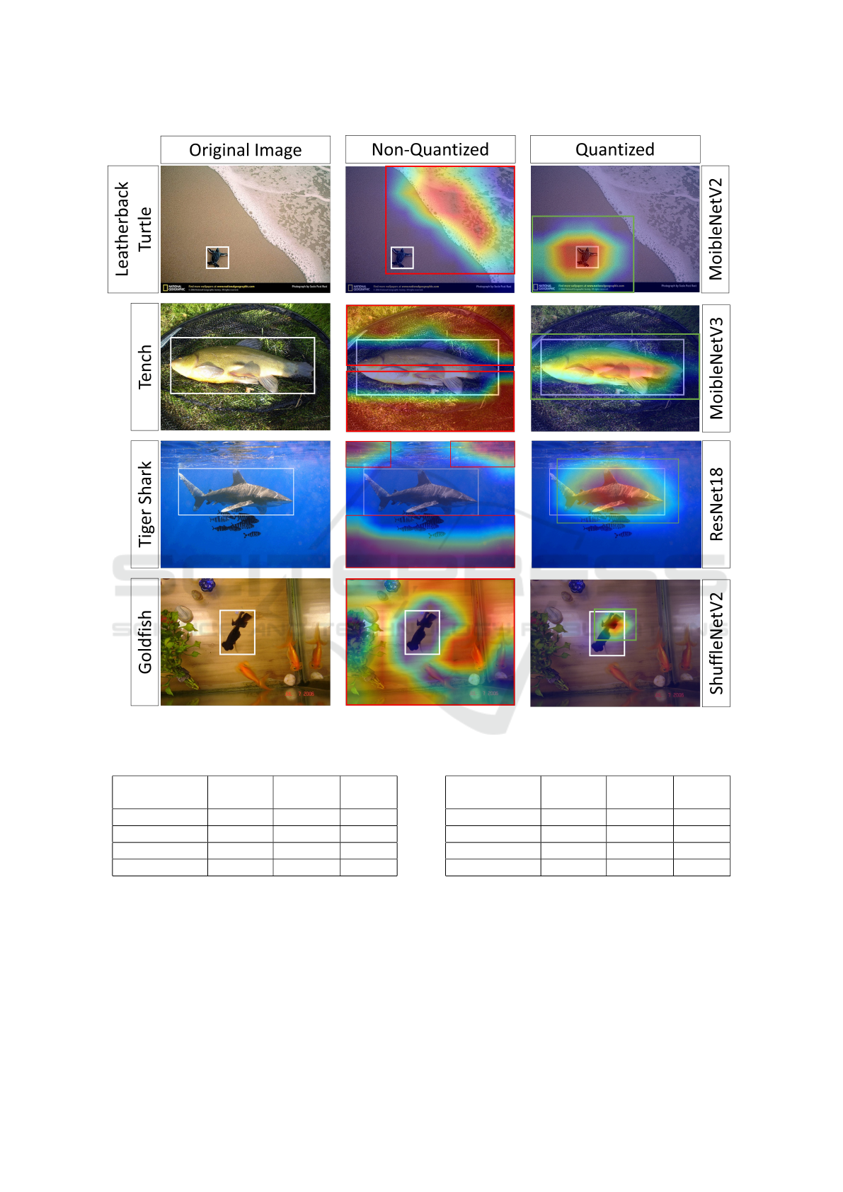
Figure 3: Comparison of Non-Quantized and Quantized CNNs, white boxes are the ground truth label, red boxes are the lower

accuracy predictions, and green boxes are higher accuracy predictions.

Table 10: Quantized CAM Evaluation.

Model

Deletion

(%)

Insertion

(%)

WSOL

(%)

MobileNetV2 0.984 10.589 30.717

MobileNetV3 1.529 32.032 26.896

ResNet18 0.496 9.244 27.942

ShufﬂeNetV2 0.289 2.613 28.845

tively. Whereas the Non-Quantized CNNs scored

30.701%, 26.790%, 27.840%, and 28.740% for the

MobileNetV2, MobileNetV3, ResNet18, and Shuf-

ﬂeNetV2, respectively. The scores for the Quan-

tized CNNs were slightly higher, with increases rang-

ing from 0.016% to 0.106% across different models

with the MobileNetV2 increasing by 0.016%, Mo-

bileNetV3 increasing by 0.106%, ResNet18 increas-

Table 11: Non-Quantized CAM Evaluation.

Model

Deletion

(%)

Insertion

(%)

WSOL

(%)

MobileNetV2 0.450 12.658 30.701

MobileNetV3 7.560 44.659 26.790

ResNet18 0.531 10.464 27.840

ShufﬂeNetV2 0.117 0.127 28.740

ing by 0.102%, and the ShufﬂenetV2 increasing by

0.105%. These results are not massive, however, they

make sense. Quantization, as mentioned, is a method

of generalization and therefore creates more general-

izable CNNs.

For a visual comparison, Figure 3 illustrates the

comparison between the Non-Quantized and Quan-

tized CAMs. In the ﬁrst column each image has a

KDIR 2023 - 15th International Conference on Knowledge Discovery and Information Retrieval

118

ground truth bounding box, in the second column is

the Non-Quantized CAM, and in the third column is

the Quantized CAM. The ﬁrst row displays a predic-

tion from MobileNetV2 on a Leatherback Turtle, the

second row shows a prediction from MobileNetV3 on

a Tench ﬁsh, the third row presents a prediction from

ResNet18 on a Tiger Shark, and ﬁnally, the fourth

row exhibits the ShufﬂeNetV2 with a prediction on

a Goldﬁsh. In each case, it is evident that the CAMs

generated by the Quantized CNNs produce more con-

cise bounding boxes for the respective images. This

observation aligns with the reported WSOL IoU val-

ues.

5 CONCLUSION

To conclude, we have visualized and statistically

compared activations from Quantized and Non-

Quantized CNNs and identiﬁed differences within the

activations themselves. Moreover, we have compared

Quantized CNN activations in a WSOL task and com-

pared the visualizations to their Non-Quantized CNN

counterparts. Through this visualization, we have

identiﬁed that Quantized CNNs utilize different fea-

tures and regions for image classiﬁcation using the

ImageNet dataset. From this, we have demonstrated

that Quantized CNNs exhibit higher performance in

WSOL tasks and can be deployed in real-time using

EigenCAM, and are statisically different. Thus, quan-

tization should be considered in more academic pa-

pers, as it not only offers a more efﬁcient network but

also provides a more interpretable network in some

cases.

For our future work, we will apply gradient-free

methodologies to activations, incorporating ViTs, in

order to explore the distinctions between Quantized

and Non-Quantized ViT models.

ACKNOWLEDGEMENTS

This work is supported by the Engineering and Phys-

ical Sciences Research Council [EP/S023917/1].

REFERENCES

Bany Muhammad, M. and Yeasin, M. (2021). Eigen-cam:

Visual explanations for deep convolutional neural net-

works. SN Computer Science, 2:1–14.

Chattopadhay, A., Sarkar, A., Howlader, P., and Balasub-

ramanian, V. N. (2018). Grad-cam++: Generalized

gradient-based visual explanations for deep convolu-

tional networks. In 2018 IEEE winter conference on

applications of computer vision (WACV), pages 839–

847. IEEE.

Ghimire, D., Kil, D., and Kim, S.-h. (2022). A survey on

efﬁcient convolutional neural networks and hardware

acceleration. Electronics, 11(6).

Gholami, A., Kim, S., Dong, Z., Yao, Z., Mahoney, M. W.,

and Keutzer, K. (2021). A survey of quantization

methods for efﬁcient neural network inference.

He, K., Zhang, X., Ren, S., and Sun, J. (2015). Deep resid-

ual learning for image recognition.

Howard, A., Sandler, M., Chu, G., Chen, L.-C., Chen, B.,

Tan, M., Wang, W., Zhu, Y., Pang, R., Vasudevan, V.,

Le, Q. V., and Adam, H. (2019). Searching for mo-

bilenetv3.

Jacob, B., Kligys, S., Chen, B., Zhu, M., Tang, M., Howard,

A., Adam, H., and Kalenichenko, D. (2017). Quan-

tization and training of neural networks for efﬁcient

integer-arithmetic-only inference.

Liang, T., Glossner, J., Wang, L., Shi, S., and Zhang,

X. (2021). Pruning and quantization for deep neu-

ral network acceleration: A survey. Neurocomputing,

461:370–403.

Liu, J., Tripathi, S., Kurup, U., and Shah, M. (2020). Prun-

ing algorithms to accelerate convolutional neural net-

works for edge applications: A survey. arXiv preprint

arXiv:2005.04275.

Ma, L., Hong, H., Meng, F., Wu, Q., and Wu, J. (2023).

Deep progressive asymmetric quantization based on

causal intervention for ﬁne-grained image retrieval.

IEEE Transactions on Multimedia, pages 1–13.

Ma, N., Zhang, X., Zheng, H.-T., and Sun, J. (2018). Shuf-

ﬂenet v2: Practical guidelines for efﬁcient cnn archi-

tecture design.

Paszke, A., Gross, S., Massa, F., Lerer, A., Bradbury, J.,

Chanan, G., Killeen, T., Lin, Z., Gimelshein, N.,

Antiga, L., Desmaison, A., Kopf, A., Yang, E., De-

Vito, Z., Raison, M., Tejani, A., Chilamkurthy, S.,

Steiner, B., Fang, L., Bai, J., and Chintala, S. (2019).

PyTorch: An Imperative Style, High-Performance

Deep Learning Library. In Wallach, H., Larochelle,

H., Beygelzimer, A., d’Alch

e Buc, F., Fox, E., and

Garnett, R., editors, Advances in Neural Information

Processing Systems 32, pages 8024–8035. Curran As-

sociates, Inc.

Petsiuk, V., Das, A., and Saenko, K. (2018). Rise: Ran-

domized input sampling for explanation of black-box

models.

Ramaswamy, H. G. et al. (2020). Ablation-cam: Vi-

sual explanations for deep convolutional network via

gradient-free localization. In proceedings of the

IEEE/CVF winter conference on applications of com-

puter vision, pages 983–991.

Russakovsky, O., Deng, J., Su, H., Krause, J., Satheesh,

S., Ma, S., Huang, Z., Karpathy, A., Khosla, A.,

Bernstein, M., Berg, A. C., and Fei-Fei, L. (2015).

ImageNet Large Scale Visual Recognition Challenge.

International Journal of Computer Vision (IJCV),

115(3):211–252.

Sabih, M., Hannig, F., and Teich, J. (2020). Utilizing ex-

Evaluating the Use of Interpretable Quantized Convolutional Neural Networks for Resource-Constrained Deployment

119

plainable ai for quantization and pruning of deep neu-

ral networks.

Sandler, M., Howard, A., Zhu, M., Zhmoginov, A., and

Chen, L.-C. (2019). Mobilenetv2: Inverted residuals

and linear bottlenecks.

Selvaraju, R. R., Cogswell, M., Das, A., Vedantam, R.,

Parikh, D., and Batra, D. (2019). Grad-CAM: Visual

explanations from deep networks via gradient-based

localization. International Journal of Computer Vi-

sion, 128(2):336–359.

Shrikumar, A., Greenside, P., and Kundaje, A. (2019).

Learning important features through propagating ac-

tivation differences.

Srinivas, S. and Fleuret, F. (2019). Full-gradient represen-

tation for neural network visualization.

Wang, H., Wang, Z., Du, M., Yang, F., Zhang, Z., Ding, S.,

Mardziel, P., and Hu, X. (2020). Score-cam: Score-

weighted visual explanations for convolutional neu-

ral networks. In Proceedings of the IEEE/CVF con-

ference on computer vision and pattern recognition

workshops, pages 24–25.

Xu, S., Huang, A., Chen, L., and Zhang, B. (2020). Con-

volutional neural network pruning: A survey. In 2020

39th Chinese Control Conference (CCC), pages 7458–

7463. IEEE.

Zee, T., Lakshmana, M., and Nwogu, I. (2022). To-

wards understanding the behaviors of pretrained com-

pressed convolutional models. In 2022 26th Inter-

national Conference on Pattern Recognition (ICPR),

pages 3450–3456. IEEE.

KDIR 2023 - 15th International Conference on Knowledge Discovery and Information Retrieval

120