A Study on the Energy Efficiency of Various Gaits for Quadruped
Robots: Generation and Evaluation
Roman Zashchitin
a
and Dmitrii Dobriborsci
b
Deggendorf Institute of Technology, 93413 Cham, Germany
Keywords:
Quadrupedal Robots, Walking Robots, Reinforcement Learning, Gait Generating.
Abstract:
This paper presents an approach for generating various types of gaits for quadrupedal robots using limb contact
sequencing. The aim of this research is to explore the capabilities of reinforcement learning in reproducing
and optimizing locomotion patterns. The proposed method utilizes the PPO algorithm, which offers improved
performance and ease of implementation. By specifying a sequence of limb contacts with the ground, gaits
such as Canter, Half bound, Pace, Rotary gallop, and Trot are generated. The analysis includes evaluating
the energy efficiency and stability of the generated gaits. The results demonstrate energy-efficient locomotion
patterns and the ability to maintain stability. The findings of this study have significant implications for the
practical application of legged robots in various domains, including inspection, construction, elderly care, and
home security. Overall, this research showcases the potential of reinforcement learning in gait generation and
highlights the importance of energy efficiency and stability in legged robot locomotion.
1 INTRODUCTION
For an extended period of time, starting from the late
20th century, scientific research has been conducted
to explore the applicability of Reinforcement Learn-
ing (RL) algorithms in the field of multidimensional
robot control, including helicopters (Bagnell and
Schneider, 2001), (Ng et al., 2003), bipeds (Zhang
and Vadakkepat, 2003), and quadrupeds (Hornby
et al., 1999). The main advantage of walking robots
over wheeled robots is the ability to move on uneven
terrain through the use of intermittent contact and the
possibility of shifting the center of mass relative to
the point of contact, which is provided by leg mech-
anisms (Kim and Wensing, 2017). All the above-
mentioned allows the use of such robots in various
areas: inspection, construction, care of the elderly,
home security, etc. Even in the early stages of studies,
the potential of automated motion generation, where
speed is an important success criterion, was demon-
strated (Kohl and Stone, 2004).
The problem formulated during that time remains
relevant to this day:
• Simplifying multidimensional control and the
process of tuning parameterized movements,
a
https://orcid.org/0009-0001-7637-5517
b
https://orcid.org/0000-0002-1091-7459
which currently require significant time and
extensive operator experience. Additionally,
changes in hardware configuration or surface
characteristics also necessitate system recalibra-
tion.
• Ensuring more efficient and optimal movements
of robotic systems.
• Improving speed, stability, energy efficiency, and
adaptability to diverse environmental conditions.
• Creating universal models applicable to different
types of robots, eliminating the need to manually
adjust gait for each specific robot.
The area of walking robots has made significant
progress in recent years, with the development of so-
phisticated hardware (Hutter et al., 2016) and control
algorithms (Hwangbo et al., 2019). However, a ma-
jor challenge remains in the ability to automatically
generate robust and efficient gaits for these robots.
This is particularly important for real-world applica-
tions, where the robots must navigate unpredictable
and complex environments.
In nature, there exists a vast variety of animal
gaits, characterized by different tempos, dynamics,
and purposes. Each of these gaits possesses its ad-
vantages and disadvantages, including high speed and
energy efficiency. This paper does not aim to find a
universal gait; instead, it employs the principles of
Zashchitin, R. and Dobriborsci, D.
A Study on the Energy Efficiency of Various Gaits for Quadruped Robots: Generation and Evaluation.
DOI: 10.5220/0012234600003543
In Proceedings of the 20th International Conference on Informatics in Control, Automation and Robotics (ICINCO 2023) - Volume 1, pages 311-319
ISBN: 978-989-758-670-5; ISSN: 2184-2809
Copyright © 2023 by SCITEPRESS – Science and Technology Publications, Lda. Under CC license (CC BY-NC-ND 4.0)
311

biomimicry to generate various gaits observed in na-
ture using reinforcement learning. Specifically, the
study examines gaits such as Canter, Half bound,
Pace, Rotary gallop, and Trot. Following the training
of the reinforcement learning algorithm using these
reference gaits, an analysis is conducted to assess the
energy efficiency of these gaits at different speeds and
evaluate the algorithm’s learning capability.
Two aspects of legged locomotion are of greater
interest in this study: dynamic physical interaction
with the environment and energy efficiency. Dynamic
locomotion requires more complex control algorithms
and is generally more challenging than static loco-
motion. It is necessary to estimate the state of the
robot: the state vector of the system, which includes
linear and angular coordinates of the torso, leg posi-
tions, rotation joint angles, etc. Then the state vec-
tor is transmitted to the control system, which is di-
rectly responsible for the coordination of all body
parts in space, generates trajectories of tool points in
the mechanism, the angle of attack, the generation of
moments on the joints, and other indicators responsi-
ble for gait and balance. The implementation of such
complexly structured and massive control systems is
often a costly and time-consuming process, due to the
description of the system by complex dependencies.
2 GAIT GENERATION METHOD
2.1 Reinforcement Learning
This paper uses a class of reinforcement learn-
ing algorithms PPO (Proximal Policy Optimization)
(Schulman et al., 2017b), which provides similar or
better performance than current approaches, but has
a simpler implementation and tuning. Supervised
learning leaves it possible to implement a cost func-
tion, use gradient descent, and get good results with
relatively little hyperparameter tuning. PPO strikes
a balance between simple implementation, sampling
complexity, and ease of tuning. The PPO function
has the form:
L
CLIP
=
ˆ
E
t
h
min

r
t
(θ)
ˆ
A
t
, clip

r
t
(θ),
1 − ε, 1 + ε

ˆ
A
t
i
, (1)
where θ is the policy parameter, E
t
- empirical expec-
tation by time steps, r
t
- probability ratio under the
new and old policy, A
t
- expected time advantage t, ε
- hyperparameter.
The PPO-Clip algorithm relies on a specialized
clipping mechanism in the objective function to pre-
vent the new policy from deviating too far from the
old policy. This approach simplifies the algorithm and
makes it compatible with stochastic gradient descent.
The algorithm has been extensively tested and has
shown excellent performance in continuous control
tasks. By removing the KL-divergence term and the
constraint, PPO-Clip streamlines the updating process
and provides incentives for the new policy to stay
close to the old policy through clipping. (Schulman
et al., 2017a).
The goal of reinforcement learning is to learn to
act in the environment in the most optimal way pos-
sible. The terminology of reinforcement learning and
optimal control is thought to be equivalent and tightly
overlapping. Optimal action in the environment is
achieved by maximizing reward rather than minimiz-
ing error.
2.2 Mechanism of Effective Gait
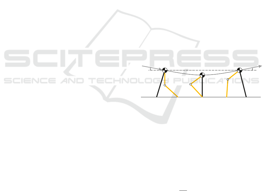
The paper (Bertram and Gutmann, 2009) pays atten-
tion to the mechanism of galloping by different ani-
mals. It is believed that the main difference between
different types of canter is in the set of limbs (hind or
forelimbs), which initiate the change of direction of
the velocity of the center of mass, during the contact
with the ground (Figure 1) (Blickhan, 1989).
–
υ
α/2
α/2
+
υ
–
υ
α/2
α/2
+
υ
Figure 1: Schematic representation of the transfer of the
center of gravity of the leg relative to the point of contact,
presented in the paper.
It is during the change of the velocity vector that
the greatest loss of momentum and kinetic energy
occurs. An important observation is that fast and
energy-efficient movement is provided only during
dynamic locomotion, when the center of mass is sta-
ble for short periods of time. Equation 2 present the
dependence of the loss of kinetic energy on the angle
of the incoming and outgoing velocity vector.
∆E
E
−
= sin
2
α ≈ α
2
. (2)
Based on equation 2, the fraction of energy lost
during the transition from one collision to another is
approximately equal to α
2
, where α is the angle be-
tween the velocity vectors v
−
and v
+
. This conclusion
is valid only for small angles and a single collision.
ICINCO 2023 - 20th International Conference on Informatics in Control, Automation and Robotics
312

(a) Canter reference and de
facto
(b) Half bound reference
and de facto
(c) Pace reference and de
facto
(d) Rotary gallop reference
and de facto
(e) Trot reference and de
facto
Figure 2: Gait diagrams showing coordination patterns for
asymmetrical gaits. Shaded bars represent stance phases,
open areas between bars represent swing phases, and num-
bered arrows show footfall timing. The yellow bars show
the reference gait and the orange bars show the gait obtained
after RL training. LH: left hind limb; RH: right hind limb;
LF: left front limb; RF: right front limb.
2.3 Reference Gaits
The book (Clayton, 2004) focuses on biomechanics,
dynamics, and various types of gaits, providing a de-
tailed description of aspects such as leg movement se-
quencing during running, depending on the phase and
its cyclic nature.
Initially, one of the primary objectives of this
study was to minimize the utilization of mathemat-
ical dependencies in gait generation. Consequently,
the mathematical description of gait, involving calcu-
lations of phase lengths, cycles, cyclic offset angles,
and other dependencies, was simplified to the spec-
ification of a sequence of limb transitions in contact
with the ground. Thus, practically all mathematical
dependencies are intended to be addressed by the RL
algorithm.
The depicted gaits in the book are illustrated in
Figure 2. Detailed explanations regarding the ob-
tained results will be presented in Section 5.
3 ALGORITHM SETTINGS
POLICY AND REWARDS
Setting up the environment involves designing a dy-
namic model of the robot and its environment. A cor-
rectly composed model must contain such parameters
as:
• Inertia tensors for each link;
• Physical constraints on the motion of links relative
to each other, including the collision of objects,
for the impossibility of bodies to intersect;
• Physical constraints on the motion of joints, in-
cluding the range of possible positions, velocities
and moments, the value of friction and damping
coefficients.
A sufficiently detailed model of ANYmal is pro-
vided by the manufacturer in URDF format in the of-
ficial Github repository, which was taken as a basis
(ANYbotics, 2023). The environment at this stage
represents a pure plateau with the global damping and
friction coefficient set.
Setting up an agent involves making up two vec-
tors of values: a state vector and a control vector. It
is important to use only the data that can be obtained
with real sensors such as inertial measurement mod-
ules, floor contact pressure sensors, position sensors,
etc. Thus, the state vector to the agent input consists
of a vector of dimension obDim = 85, and the output
of dimension actionDim = 12, equal to the number
of motors of the robot. The output vector generates
torque values for each robot motor. Other methods of
motion control are also possible, such as force con-
trol, position control, and velocity-based control.
Computer simulators are physically unable to sim-
ulate the real physics of contact interaction and are
only approximate (Hwangbo et al., 2018), and ma-
chine learning algorithms themselves often find a
loophole in the simulator and exploit this inaccuracy.
The simulation model of the robot itself, the dynam-
ics, and the coefficient values are also approximate
and imply some deviations in the final result of the
walking robot. Based on the presented disadvantages
of the resulting gait, it becomes necessary to formu-
late additional rewards.
We have been inspired by the award functions in
the papers (Hwangbo et al., 2019), (Lee et al., 2020),
(Miki et al., 2022), in developing the functions needed
to meet the goals of this paper. The rewards used dur-
ing training can be divided into several categories that
solve a particular problem during gait generation.
In this paper, several experimental rounds are pre-
sented, consisting of a combination of soft and hard
constraints.
Soft constraints are primarily implemented using
reward functions and the assignment of appropriate
coefficients. Such constraints on the solution search
space allow for gait adaptation to the robot’s dy-
namic characteristics if a specific gait cannot be used
A Study on the Energy Efficiency of Various Gaits for Quadruped Robots: Generation and Evaluation
313

without modifications. The algorithm is designed to
independently establish dependencies between cycle
length, contacts, flight, and phase lengths based on the
specified movement speed along the ˆx and ˆy plane.
To achieve realistic movements and enhance the
algorithm’s applicability to a physical robot, we intro-
duce rewards that are inversely correlated with metric
minimization:
• The error between the actual linear velocity and
the given linear velocity command.
• The error between the actual angular velocity
command and the given angular velocity com-
mand.
• The generated torque of the actuators.
• The speed of the actuators.
• Limb lift relative to the point of contact with the
floor and slippage.
• Step changes in speed and torque of the actuators.
• Roll, pitch, and yaw angles of the main body of
the robot.
• The robot’s center of mass at a certain height.
• The phase time when the limbs are not in contact
with the floor.
• The robot’s velocity in space along the ˆz axis.
• The error in following the reference gait (op-
tional).
Hard constraints serve as an extension to the soft
constraints, representing a set of episode interruption
functions that are triggered if the robot exceeds the
permissible limits during a specified time. For in-
stance:
• Interrupting the episode if contact between the
robot and the ground was not made by the robot’s
leg;
• Interrupting the episode if the robot’s body ge-
ometric center excessively deviates along the z-
axis, relative to the specified position;
• Interrupting the episode if the robot’s body yaw
deviates excessively from the zero value while
running in a straight line;
• Interrupting the episode if the robot’s coordi-
nates reach manually set, non-recommended val-
ues while running in a straight line.
Hard constraints are imposed to significantly re-
duce the search space, consequently decreasing the
training time. However, with hard constraints in
place, the debugging time for reward functions in-
creases, as the training convergence time is noticeably
extended.
3.1 Hyperparameters for PPO
The tuning of hyperparameters in the PPO algorithm
for reinforcement learning is an essential part of the
training process. Hyperparameters, such as learning
rate, minibatch size, and the number of optimization
epochs, determine various aspects of the algorithm.
Making the right choices for these hyperparameters
can enhance the performance and efficiency of the
algorithm, ensuring faster and more stable conver-
gence towards an optimal policy. However, determin-
ing the optimal values for hyperparameters requires
experimentation and thorough investigation. Achiev-
ing this optimization can significantly impact the al-
gorithm’s effectiveness and contribute to the advance-
ment of reinforcement learning techniques (Godbole
et al., 2023). The parameters used in the training are
presented in Table 1.
Table 1: Hyperparameters for PPO.
Value
learning rate 5e-4
discount factor 0.998
learning epoch 4
GAE-lambda 0.95
clip ratio 0.2
entropy coefficient 0.0
batch size 4
3.2 Logistic Kernel
We use a logistic kernel to define a bounded cost
function. This kernel converts a tracking error to a
bounded reward. The logistic kernel ensures that the
cost is lower-bounded by zero and termination be-
comes less favorable.
Logistic Kernel(LK) : R → [−0.25, 0) as
LK(x) =
−1
exp
x
+2 + exp
−x
(3)
3.3 Reward Functions
The process of tuning reward functions in reinforce-
ment learning for robotic systems was carried out
in a systematic and iterative manner. Initially, a
small number of rewards and their corresponding
adjustments were considered. As the process ad-
vanced, more sophisticated functions were incorpo-
rated to enhance the performance of the robotic sys-
tem, and these changes were reinforced through mul-
tiple rounds of experimentation. These experiments
served to verify the functionality of the system and
tackle a variety of challenges, such as RL algorithm
ICINCO 2023 - 20th International Conference on Informatics in Control, Automation and Robotics
314

attempts to exploit vulnerabilities in the simulator’s
physical engine, unrealistic robot movements, among
other issues.
The dynamic locomotion of a complex robotic
system featuring 12 degrees of freedom presents a
vast and intricate space of potential configurations.
Due to the enormity of this space, searching for feasi-
ble gaits in all possible configurations is not a practi-
cal approach. To optimize the system’s performance,
it is essential to strike a balance between an excessive
search space and an insufficient one. It is possible that
the optimal policy for the task at hand may not have
been identified within 25,000 epochs. However, the
primary experimental trends can often be observed,
providing valuable insights into the system’s behav-
ior and potential improvements.
To further refine the search process, randomly
generated initial points within the search space can
be mitigated by increasing the number of trial rounds
and training iterations. Interestingly, the best check-
point is not always the final one in the training pro-
cess. In this study, we actively monitor and track the
best checkpoints observed during the course of train-
ing.
Upon completion of the training process, the se-
lection of the most suitable model involves identify-
ing the optimal checkpoint observed during the train-
ing. This strategy, known as retrospective optimal
checkpoint selection, allows for a more robust and ef-
ficient choice, ultimately enhancing the performance
and capabilities of the robotic system.
The reward function is defined as:
r
f inal
= 130r
bv
+r
bw
−10(r
jτ
+r
jv
)−100(r
f c
+r
f s
)−
− 0.1r
s
− 1000r
bo
+ 0.2r
at
− 0.1r
za
+ 0.5r
gg
. (4)
The individual terms are defined as follows.
• Linear Velocity (r
bv
): This term encourages the
policy to follow a desired horizontal velocity (ve-
locity in ˆx and ˆy plane) command:
r
bv
= c
v1
LK(|c
v2
· (v
f act
− v
des
)|), (5)
where c
v1
= −10∆t, c
v2
= −4∆t, v = [v
x
, v
y
, v
z
]
T
.
• Angular Velocity (r
bω
): This term encourages the
policy to follow a desired yaw velocity command:
r
bω
= c
ω
LK(|w
f act
− w
des
|), (6)
where c
ω
= −6∆t, w = [w
x
, w
y
, w
z
]
T
.
• Joint Torque (r
jτ
): We penalize the joint torques
to reduce energy consumption:
r
jτ
= c
τ
12
∑
i=1
τ
2
i
, (7)
where c
τ
= 0.0005∆t.
• Joint Speed (r
jv
): We penalize the joint speed to
reduce jerks and add smoothness to the robot’s
movements:
r
jv
= c
v j
12
∑
i=1
v
2
j
i
, (8)
where c
v j
= 0.003∆t.
• Foot Clearance (r
f c
): We penalize the foot in the
swing phase for raising the foot too high:
r
f c
= c
f cc
4
∑
i=1

(p
des
f ,i
− p
f act
f ,i
)
2
− v
2
f ,i

, (9)
where c
f cc
= 0.1∆t.
• Foot Slip (r
f s
): We penalize the foot velocity if
the foot is in contact with the ground to reduce
slippage:
r
f s
= c
v f
4
∑
i=1
v
2
f ,i
, (10)
where c
v f
= 2.0∆t.
• Smoothness (r
s
): We penalize sudden changes in
speed and torque on the actuators, to reduce vibra-
tion and maintain realism of movement:
r
s
= c
sc
12
∑
i=1
((τ
i,t
−τ
i,t−1
)
2
+(v
i,t
−v
i,t−1
)
2
), (11)
where c
sc
= 0.04∆t.
• Body Orientation (r
bo
): We penalize for devia-
tions of pitch and roll of the robot body from zero
values and deviations of the body center height
from the set value:
r
bo
= c
boc

θ
x
+ θ
y
+ (p
f act
b,z
− p
des
b,z
)
2

, (12)
where c
boc
= 0.04∆t.
• Air Time (r
at
): We reward the agent with a long
swing phase, but impose a penalty if the swing
phase is too long to avoid excluding the limbs
from the gait:
r
at
=
=









c
atc
∑
4
i=1
((t
f ,i
− 0.5) − exp
t
f ,i
),
i f t
f ,i
> 1.5
c
atc
∑
4
i=1
(t
f ,i
− 0.5),
i f t
f ,i
≤ 1.5
(13)
where c
atc
= 2.0∆t.
A Study on the Energy Efficiency of Various Gaits for Quadruped Robots: Generation and Evaluation
315

• Body z Acceleration (r
za
): We penalize the accel-
eration of the robot’s body along the z-axis:
r
za
=
v
bz,t
− v
bz,t−1
∆t
. (14)
• Gait Generation (r
gg
): We award an agent for
Compliance with reference sets of consistent
limb-to-ground contacts:
r
gg
=
(
1, i f C
f act
f
= C
des
f
0, otherwise.
(15)
3.4 Abort Functions
• Wrong contact
1, 2, 3
:
(
True, i f C
ground,t
∈ C
f oot
False, otherwise,
(16)
where C
ground,t
- set of objects in contact with the
surface at a given moment in time, C
f oot
- set of
objects that are allowed to interact with the floor
surface.
• Exceeding height
1, 2, 3
:
(
True, i f p
init
b,z
− 0.2 < p
f act
b,z
< p
init
b,z
+ 0.1
False, otherwise.
(17)
• Exceeding yaw
1, 3
:
(
True, i f |θ
z
| < 60
◦
False, otherwise.
(18)
• Exceeding yaw
2
:
(
True, i f |θ
z
| < 40
◦
False, otherwise.
(19)
• Exceeding x and y coordinates
2
:
(
True, i f p
b,x
< −0.3 or |p
b,y
| > 0.1
False, otherwise.
(20)
4 ENERGY EFFICIENCY
CRITERIA
It is common to measure the Cost of Transport
(CoT) coefficients to study legged robots’ energy-
efficiency. CoT is a coefficient that quantifies the
1
This interrupt function is used when teaching with soft
constraints.
2
This interrupt function is used when teaching with hard
constraints.
3
This interrupt function is used in the final CoT mea-
surements.
energy-efficiency of the movement of animals, hu-
mans, or robots
CoT =
E
mgd
, (21)
where E is the energy required to transfer a body
with mass m over a distance d, and g is the gravity
constant. The smallest CoT means the most energy-
efficient motion.
To measure the energy consumed by robots during
movement, the energy measurement method for actu-
ators was used (Folkertsma et al., 2018). This method
is necessary to measure the amount of energy supplied
by the actuators to the system, i.e., the entire structure
robot.
By this method, it is possible to accurately esti-
mate the energy supplied by the controller to the mo-
tors if two conditions are satisfied: first, the actua-
tor force is constant during each moment of time, and
second, the position sensor is aligned with the actua-
tor.
When these conditions are satisfied, it is possible
to calculate the energy arriving at each moment of
time (Zashchitin et al., 2020) in the system, where the
energy in the system is equal to the internal product
of the force by the difference of discrete positions:
E =
Z
t
i+1
t
i
P(t)dt =
Z
t
i+1
t
i
⟨F(t), v(t)⟩dt =
= ⟨F(t
i
), q(t
i
+ 1) − q(t
i
)⟩, (22)
where P(t) the supplied power, F(t) and v(t) = ˙q(t)
the motor force and velocity, respectively, and q(t
i
)
the motor position at time step t
i
. Writing the discrete-
time equations in computable form, since eq. 22
needs a motor position from a future time step, where
¯
F
i−1
is the control; force set at t
i−1
and held constant
until t
i
. The energy estimate in the system can be cal-
culated using the equation:
ˆ
E
i
=
ˆ
E
i−1
+
¯
F
i−1
(q
i
− q
i−1
). (23)
in which
ˆ
E
i
is the energy estimate at time t
i
.
5 RESULTS
The duration of each test run lasts 10 seconds. The
trained models are run step by step with the given
command(horizontal x and y velocity, yawrate) {3, 0,
0}, {2, 0, 0}, {1, 0, 0} and measuring CoT. The re-
sults of CoT measurements of policies with soft con-
straints are shown in the Table 2. It can be seen that
with successful simulation completions, the CoT val-
ues come quite close to the value of 1.2, which is the
ICINCO 2023 - 20th International Conference on Informatics in Control, Automation and Robotics
316

reference (He and Gao, 2020). Despite the stabil-
ity and convergence of the policies, the final testing
demonstrates instability of the gaits and outliers in al-
most half of the cases.
A set of RL plots with a soft set of constraints is
shown in Figure 3. Based on the graphs we can note
the stability, the trend of how well the agent learns and
converges to the optimal policy. Here we can argue
that the last control point is one of the most optimal
policies.
A set of RL plots with a hard set of constraints
is shown in Figure 4. It is noticeable that the con-
vergence of learning is faster, but is unstable. The
judgement here is valid that the best control point is
not always the end point in the learning process.
Upon completion of the training process, the se-
lection of the most suitable model involves identify-
ing the optimal checkpoint observed during the train-
ing. This strategy, known as retrospective optimal
checkpoint selection, allows for a more robust and ef-
ficient choice, ultimately enhancing the performance
and capabilities of the robotic system. Table 3 shows
the CoT values of policies trained with hard con-
straints. It is evident from this series of experiments
that nearly all iterations were executed successfully;
however, the corresponding CoT values were found to
be elevated, indicating reduced energy efficiency. It is
plausible that the application of a subsequent round
of supplementary training, akin to the methodolo-
gies employed in (Bengio et al., 2009) and (Hwangbo
et al., 2019), will likely rectify this issue and yield a
more precise optimization.
Returning to the topic of gaits Section 2.3, it can
be noted that if the reference gait is not specified, the
policy defaults to a trot gait 2(e) in the case of soft
constraints or a canter gait 2(a) in the case of hard
constraints, or it resorts to a gait that utilizes inac-
curacies in the physical modeling of the mechanism.
As mentioned before, the RL algorithm will strive to
replicate the given reference gaits or adapt them to
suit its own construction peculiarities like in 2(d). In
other cases, the gaits were formed correctly.
To reproduce and review the results, please follow
the link provided (Zashchitin and Dobriborsci, 2023).
6 CONCLUSIONS
In this work, we have presented an approach for gen-
erating various types of gaits for quadrupedal robots
by specifying a sequence of limb contacts with the
ground. The study has demonstrated the capability to
generate gaits such as Canter, Half bound, Pace, Ro-
tary gallop, and Trot. The proposed method, utilizing
Table 2: CoT of different robot gaits depending on the given
command under soft constraints. Green cells in the table in-
dicate successful completion of the simulation without ex-
ceeding the permissible values. Conversely, orange cells
mean unsuccessful completion of the simulation with ex-
ceeding the permissible values.
Command {3, 0, 0} {2, 0, 0} {1, 0, 0}
CoT
Canter 1.35 1.41 1.55
Half bound 1.40 1.48 1.61
Pace 1.42 1.47 1.57
Rotary gallop 1.42 1.46 1.57
Trot 1.36 1.36 1.41
Without
gait reference
1.18 1.24 1.41
Table 3: CoT of different robot gaits depending on the given
command under hard constraints. Green cells in the ta-
ble indicate successful completion of the simulation with-
out exceeding the permissible values. Conversely, orange
cells mean unsuccessful completion of the simulation with
exceeding the permissible values.
Command {3, 0, 0} {2, 0, 0} {1, 0, 0}
CoT
Canter 1.49 1.5 1.55
Half bound 1.41 1.47 1.62
Pace 1.61 1.58 1.63
Rotary gallop 1.48 1.5 1.65
Trot 1.5 1.49 1.60
Without
gait reference
1.46 1.47 1.60
the RL algorithm PPO, offers improved performance
with simpler implementation and setup. The intro-
duced reward functions simplify, expedite, and auto-
mate the process of generating different types of gaits,
including energy-efficient and high-speed gaits.
After generating the gaits, an analysis was con-
ducted to evaluate their energy efficiency and stabil-
ity. The assessment of energy efficiency demonstrated
that the proposed method achieves energy-efficient
gaits, contributing to the optimization of robotic lo-
comotion in terms of power consumption and overall
energy expenditure. Additionally, the stability analy-
sis revealed that the obtained gaits exhibit robustness
and reliability, maintaining their desired patterns.
The results have shown the stability of the pro-
posed method even with a small number of epochs,
making it suitable for real-world deployment on
legged robot platforms. These findings highlight the
potential of the approach in various applications, such
as inspection, construction, elderly care, and home se-
curity.
Overall, our approach provides valuable insights
into gait generation for legged robots, showcasing the
A Study on the Energy Efficiency of Various Gaits for Quadruped Robots: Generation and Evaluation
317

(a) Graph of the dependence of the logarithm of the
learning rate on the number of epochs.
(b) Graph of the dependence of the logarithm of the mean
standard deviation of noise on the number of epochs.
(c) Graph of the surrogate loss function dependence on the
number of epochs.
(d) Graph of the value function estimation dependence
during training on the number of epochs.
Figure 3: An overview of the key metrics of the reinforcement learning process in the PPO algorithm with soft constraints.
(a) Graph of the dependence of the logarithm of the
learning rate on the number of epochs.
(b) Graph of the dependence of the logarithm of the mean
standard deviation of noise on the number of epochs.
(c) Graph of the surrogate loss function dependence on the
number of epochs.
(d) Graph of the value function estimation dependence
during training on the number of epochs.
Figure 4: An overview of the key metrics of the reinforcement learning process in the PPO algorithm with hard constraints.
ICINCO 2023 - 20th International Conference on Informatics in Control, Automation and Robotics
318

ability to generate stable, energy-efficient, and versa-
tile gaits. By combining reinforcement learning and
limb contact sequencing, we have demonstrated the
applicability of legged robots in diverse scenarios.
The analysis of energy efficiency and stability further
reinforces the significance of this approach and its po-
tential for practical implementation. Future research
may focus on optimizing gait patterns, incorporating
dynamic environments, and considering robustness to
varying terrains, thereby expanding the capabilities
and applications of legged robots.
REFERENCES
ANYbotics (2023). ANYmal - Autonomous Legged Robot
GitHub. https://github.com/ANYbotics.
Bagnell, J. and Schneider, J. (2001). Autonomous he-
licopter control using reinforcement learning pol-
icy search methods. International Conference on
Robotics and Automation.
Bengio, Y., Louradour, J., Collobert, R., and Weston, J.
(2009). Curriculum learning. In Proceedings of the
26th Annual International Conference on Machine
Learning, ICML ’09, page 41–48, New York, NY,
USA. Association for Computing Machinery.
Bertram, J. E. and Gutmann, A. (2009). Motions of the run-
ning horse and cheetah revisited: Fundamental me-
chanics of the transverse and rotary gallop. Journal of
the Royal Society Interface, 6(35):549–559.
Blickhan, R. (1989). The spring-mass model for run-
ning and hopping. Journal of biomechanics, 22 11-
12:1217–27.
Clayton, H. (2004). The Dynamic Horse A Biomechanical
Guide to Equine Movement and Performance. Sport
Horse Publications.
Folkertsma, G. A., Groothuis, S. S., and Stramigioli, S.
(2018). Safety and guaranteed stability through em-
bedded energy-aware actuators. In 2018 IEEE In-
ternational Conference on Robotics and Automation
(ICRA), pages 2902–2908.
Godbole, V., Dahl, G. E., Gilmer, J., Shallue, C. J., and
Nado, Z. (2023). Deep learning tuning playbook. Ver-
sion 1.0.
He, J. and Gao, F. (2020). Mechanism, actuation, per-
ception, and control of highly dynamic multilegged
robots. Chinese Journal of Mechanical Engineering
(English Edition), 33.
Hornby, G. S., Fujita, M., Takamura, S., Yamamoto, T.,
and Hanagata, O. (1999). Autonomous evolution of
gaits with the sony quadruped robot. In Proceedings
of the 1st Annual Conference on Genetic and Evolu-
tionary Computation - Volume 2, GECCO’99, page
1297–1304, San Francisco, CA, USA. Morgan Kauf-
mann Publishers Inc.
Hutter, M., Gehring, C., Jud, D., Lauber, A., Belli-
coso, C. D., Tsounis, V., Hwangbo, J., Bodie, K.,
Fankhauser, P., Bloesch, M., Diethelm, R., Bachmann,
S., Melzer, A., and Hoepflinger, M. (2016). Anymal
- a highly mobile and dynamic quadrupedal robot. In
2016 IEEE/RSJ International Conference on Intelli-
gent Robots and Systems (IROS), pages 38–44.
Hwangbo, J., Lee, J., Dosovitskiy, A., Bellicoso, D., Tsou-
nis, V., Koltun, V., and Hutter, M. (2019). Learning
agile and dynamic motor skills for legged robots. Sci-
ence Robotics, 4(26):eaau5872.
Hwangbo, J., Lee, J., and Hutter, M. (2018). Per-contact
iteration method for solving contact dynamics. IEEE
Robotics and Automation Letters, 3(2):895–902.
Kim, S. and Wensing, P. M. (2017). Design of Dynamic
Legged Robots. Foundations and Trends in Robotics,
5(2):117–190.
Kohl, N. and Stone, P. (2004). Policy gradient reinforce-
ment learning for fast quadrupedal locomotion. In
IEEE International Conference on Robotics and Au-
tomation, 2004. Proceedings. ICRA ’04. 2004, vol-
ume 3, pages 2619–2624 Vol.3.
Lee, J., Hwangbo, J., Wellhausen, L., Koltun, V., and Hut-
ter, M. (2020). Learning quadrupedal locomotion over
challenging terrain. CoRR, abs/2010.11251.
Miki, T., Lee, J., Hwangbo, J., Wellhausen, L., Koltun, V.,
and Hutter, M. (2022). Learning robust perceptive lo-
comotion for quadrupedal robots in the wild. Science
Robotics, 7(62):eabk2822.
Ng, A., Kim, H. J., Jordan, M., and Sastry, S. (2003). Au-
tonomous helicopter flight via reinforcement learning.
Advances in Neural Information Processing Systems
17.
Schulman, J., Klimov, O., Wolski, F., Dhariwal, P., and
Radford, A. (2017a). Proximal Policy Optimization.
Schulman, J., Wolski, F., Dhariwal, P., Radford, A., and
Klimov, O. (2017b). Proximal policy optimization al-
gorithms. CoRR, abs/1707.06347.
Zashchitin, R. and Dobriborsci, D. (2023). Gait-
Generation2023. https://github.com/thd-research/
code-2023-study-quadruped-gait. Accessed: 2023-
07-01.
Zashchitin, R. A., Borisov, I. I., Borisova, O. V., and Kolyu-
bin, S. A. (2020). Energy-efficiency in legged robots
locomotion: Open versus closed chains. In 2020 In-
ternational Conference Nonlinearity, Information and
Robotics (NIR), pages 1–6.
Zhang, R. and Vadakkepat, P. (2003). An evolution-
ary algorithm for trajectory based gait generation of
biped robot. Proceedings of the International Con-
ference on Computational Intelligence, Robotics and
Autonomous Systems.
A Study on the Energy Efficiency of Various Gaits for Quadruped Robots: Generation and Evaluation
319