Offline Feature-Based Reinforcement Learning with Preprocessed Image
Inputs for Liquid Pouring Control
Stephan Pareigis
1 a
, Jesus Eduardo Hermosilla-Diaz
2 b
, Jeeangh Jennessi Reyes-Montiel
2 c
,
Fynn Luca Maaß
3 d
, Helen Haase
1
, Maximilian Mang
1
and Antonio Marin-Hernandez
2 e
1
Department of Computer Science, HAW Hamburg, Berliner Tor 7, 20099 Hamburg, Germany
2
Artificial Intelligence Research Institute, Universidad Veracruzana, Calle Paseo No. 112, Xalapa, Mexico
3
Department of Computer Science, Graz University, 8010 Graz, Inffeldgasse 16, Austria
Keywords:
Offline Reinforcement Learning, Pouring Liquid, Artificial Neural Network, Robust Control, UR5 Robot
Manipulator.
Abstract:
A method for the creation of a liquid pouring controller is proposed, based on experimental data gathered from
a small number of experiments. In a laboratory configuration, a UR5 robot arm equipped with a camera near
the end effector holds a container. The camera captures the liquid pouring from the container as the robot
adjusts its turning angles to achieve a specific pouring target volume.
The proposed controller applies image analysis in a preprocessing stage to determine the liquid volume pouring
from the container at each frame. This calculated volume, in conjunction with an estimated target volume in
the receiving container, serves as input for a policy that computes the necessary turning angles for precise
liquid pouring. The data received on the physical system is used as Monte-Carlo episodes for training an
artificial neural network using a policy gradient method.
Experiments with the proposed method are conducted using a simple simulation. Convergence proves to be
fast and the achieved policy is independent of initial and goal volumes.
1 INTRODUCTION
Developing an optimal control for a non-linear sys-
tem usually requires a detailed model of the plant or
process. Reinforcement learning (Sutton and Barto,
2018) is a method used to develop a controller, pro-
vided the controlling agent has the opportunity to
search and experiment with different actions, receiv-
ing respective rewards.
Creating sufficiently detailed models of the sys-
tem to be controlled is often costly and difficult. Often
times, the optimal control (policy) developed using a
simulation of the system does not work in practice
due to imprecise modeling of the system dynamics
and sensor data.
There are different approaches to mitigate the so-
a
https://orcid.org/0000-0002-7238-0976
b
https://orcid.org/0009-0001-0575-5096
c
https://orcid.org/0000-0003-3194-914X
d
https://orcid.org/0000-0002-4555-4870
e
https://orcid.org/0000-0002-7697-9118
called simulation to reality gap (Zhao et al., 2020).
One method may be to explicitly simulate the sim-to-
reality gap, i.e. by including artificial sensor noise.
However, this requires detailed knowledge about the
system as a whole to anticipate possible differences
between the simulation and the physical system.
Given this problem, it is usually better to collect
data and run experiments directly within the physical
system. However, this is usually not possible because
physical systems are often much slower than simu-
lations and therefore a large number of experiments
cannot be carried out, as is often needed in reinforce-
ment learning. In addition, safety aspects often play a
role, for example in autonomous driving, robotics or
aviation.
Strategies to cope with the problem that simula-
tions sometimes lack necessary precision and phys-
ical systems lack proper speed to run many experi-
ments, have been developed. Methods are used in
which a teacher demonstrates the experiments. In-
verse reinforcement learning (IRL) (Arora and Doshi,
2021), for example, tries to derive a reward function
320
Pareigis, S., Hermosilla-Diaz, J., Reyes-Montiel, J., Maaß, F., Haase, H., Mang, M. and Marin-Hernandez, A.
Offline Feature-Based Reinforcement Learning with Preprocessed Image Inputs for Liquid Pouring Control.
DOI: 10.5220/0012235700003543
In Proceedings of the 20th International Conference on Informatics in Control, Automation and Robotics (ICINCO 2023) - Volume 1, pages 320-326
ISBN: 978-989-758-670-5; ISSN: 2184-2809
Copyright © 2023 by SCITEPRESS – Science and Technology Publications, Lda. Under CC license (CC BY-NC-ND 4.0)

from the demonstrations and use it to train a con-
troller.
We introduce a laboratory setup in which a few
predefined experiments are carried out in the task of
pouring liquids. The data from those experiments is
stored accordingly as described in section 3.1. Later,
this data is used to train a reinforcement learning con-
troller in an offline manner. As the training algorithm
does not have direct access to the system, exploration
becomes impossible.
In the given laboratory setup, a camera is mounted
on top of the end effector of a UR5 robot arm. A con-
tainer with a liquid is held in the end effector. The task
is to turn the end effector such that a precise volume
of liquid is poured out. The system therefore con-
sists of a camera image as input space, and angles of
the end effector (one-dimensional) as output space. A
maximal reward is awarded if a given output volume
is met precisely.
The proposed controller uses two steps: In the first
step, the camera image is analyzed using image pro-
cessing software. A measure for the liquid quantity
leaving the container is calculated. This measure can
be considered to be a feature of the liquid as seen in
the image.
In the second step, this feature is input into an ar-
tificial neural network (ANN) that serves as a policy
model for determining pouring angles. This two-step
process, utilizing pre-processed images, offers the ad-
vantage of a reduced input dimension for the ANN.
Consequently, a smaller ANN can be selected, re-
sulting in faster training and inference compared to
a high-dimensional input space.
As action space, we use discretized relative turn-
ing angles of the end effector. The fact that the an-
gles are chosen to be relative enables the method
to be independent of the initial volume in the pour-
ing container. This approach of relative and dis-
cretized rotation angles uses our idea from robust au-
tonomous driving, as we presented in (Pareigis and
Maaß, 2023).
There are a variety of publications on pouring liq-
uid. We just mention a few which are closely related
to our approach.
(Schenck and Fox, 2017) presents a solution for
pouring specific amounts of liquids based on imagery,
independent of the initial volume of liquid in the
source container. A camera films the target container
and the images are fed into a two-stage neural net-
work.
(Moradi et al., 2021) apply Soft Actor-Critic
(SAC) with an Convolutional Neural Network (CNN)
as a reward approximate. The task containes pick-
ing up, moving and pouring the entire liquid from one
container to another.
An alternative approach employing the Actor-
Critic method is presented by (Tamosiunaite et al.,
2011). They integrate goal learning through an ap-
proximate function and shape learning using a Non-
linear Autoencoder (NAC) and a Probabilistic Infer-
ence Optimization (PI2) technique.
While the approaches mentioned earlier demon-
strate success within their specific contexts, chal-
lenges arise when applying them in real-world sce-
narios. For instance, the method proposed by (Ta-
mosiunaite et al., 2011) relies on prior knowledge of
the robot’s liquid quantity, which can vary. To ad-
dress this limitation, we will employ discretized rela-
tive angles as action space, ensuring that the pouring
process remains independent of the initial volume in
the source container.
Another limitation of both (Schenck and Fox,
2017) and (Moradi et al., 2021) is their reliance on
volume estimation of liquid in the recipient container
through imagery. Consequently, it becomes essen-
tial that the recipient container remains visible from
a specific angle or is transparent to allow for accurate
liquid volume assessment. This requirement parallels
related research on estimating liquid volumes from
single images, as observed in works such as (Cobo
et al., 2022) and (Liu et al., 2023).
The benefit of just observing the liquid flowing
out of the source container as in the proposed setup
is, that it can be poured into not or only partially ob-
servable containers. Additionally, it could be poured
onto surfaces or soils, where no accumulation of
liquid would be visible, for example when watering
plants.
The experimental setup is described in section 2.
Section 3 describes the proposed algorithm in three
steps: Data acquisition in section 3.1, the controller
architecture in section 3.2, and training the controller
in section 3.3. Simple experiments were performed
which are described briefly in section 4. Section 5
concludes with a summary and remarks on current
work.
2 EXPERIMENTAL SETUP AND
REQUIREMENTS
A UR5 robot manipulator is equipped with an end ef-
fector holding a container, denoted as C, containing
an initial liquid volume of V
init
. As the end effector is
rotated, the liquid pours out. It is assumed that the re-
ceiving container, designated as R, is adequately sized
to capture all of the poured liquid.
Offline Feature-Based Reinforcement Learning with Preprocessed Image Inputs for Liquid Pouring Control
321

In Figure 1, the side view of the setup is illus-
trated, along with a reference coordinate system. The
Intel RealSense camera is mounted on the robotic
wrist and is aligned to capture a continuous video of
the liquid as it exits the container.
Figure 2 shows the system from the top and from
the front.
Figure 1: A local reference framework, denoted as O
L
, is
positioned at the center of the container base. The wrist is
initially in position 0
◦
.
(a) (b)
Figure 2: Experimental design: a) top view of the materials
used and b) front view of the pouring process.
The goal is to pour out a certain volume V
G
of liq-
uid. This requires an appropriate function α(t) for
steering the angle of the end effector in time. This
function cannot be computed ahead of time (open
loop control) because the initial volume of the liquid
in the container C is not known.
Consequently, container C needs to be rotated un-
til the liquid starts pouring out of it. Based on the vol-
ume observed by the camera positioned atop the end
effector, the angle α must be continuously adjusted as
to meet the desired goal volume, denoted as V
G
.
A scale is used to measure the weight w of the liq-
uid in the receiving container R at the end of the pour-
ing sequence. This way, the received volume of the
liquid can be measured within a certain precision. The
current weight of the liquid on the scale may not be
used in real-time in the feedback algorithm. It is as-
sumed that the scale may only be read after the pour-
ing process. The reason for this is that an ordinary
kitchen scale is used which has a delay and no digital
output.
It is furthermore assumed, that a simulation of the
setup is not available within a reasonable precision.
Only basic experiments with the real setup can be per-
formed. These experiments will take some time and
are slow to perform. However, experiments with the
real setup provide a ground truth dependency between
images, pouring angles and output volume.
The task shall be to design a set of experiments
with the laboratory setup and use this data in an offline
manner to develop a controller which will then be able
to pour out liquids with a given goal volume V
G
.
3 CONTROLLER
ARCHITECTURE
First, the method to collect data from the real labora-
tory setup is described. In section 3.2 the architecture
of the controller is presented. Section 3.3 describes
the training and setup of the controller.
3.1 Data Acquisition
The laboratory setup as shown in figure 2 is prepared
with an arbitrary amount V
init
of initial liquid in the
container C inside the gripper of the UR5. The angle
α is initially set to 0. The recipient (a regular coffee
cup) is initially empty and the scale is set to zero.
A pre-programmed movement of the end effector
is applied. The movement results from the function
α(t) := λ ·e
−(γ·(t−β)
2
)
(1)
applied to the angle of the end effector. λ, γ and
β are parameters to change the height and duration of
the curve. Figure 3 shows different angle curves in
time for various parameters λ, γ and β.
Basically, any kind of angle curve in time which
starts at angle 0 and returns to angle 0 could be used
for these experiments, e.g. λsin(γ·t). However, equa-
tion (1) has the advantage that the acceleration is slow
so as not to create unnecessary turbulence in the liquid
while pouring out.
After returning to zero, the resulting weight on the
scale is read and registered. Subsequently, one single
experiment consisting of a sequence of angles, cam-
era frames and a resulting weight shall be called ex-
perimental episode E.
During each experimental episode the images
taken from the camera together with the respective an-
gle α are stored. This way each experimental episode
E leads to a list L
E
of the following format:
L
E
= {(Image
i
, α(i))| i = 0, 1, 2,· ··}.
ICINCO 2023 - 20th International Conference on Informatics in Control, Automation and Robotics
322

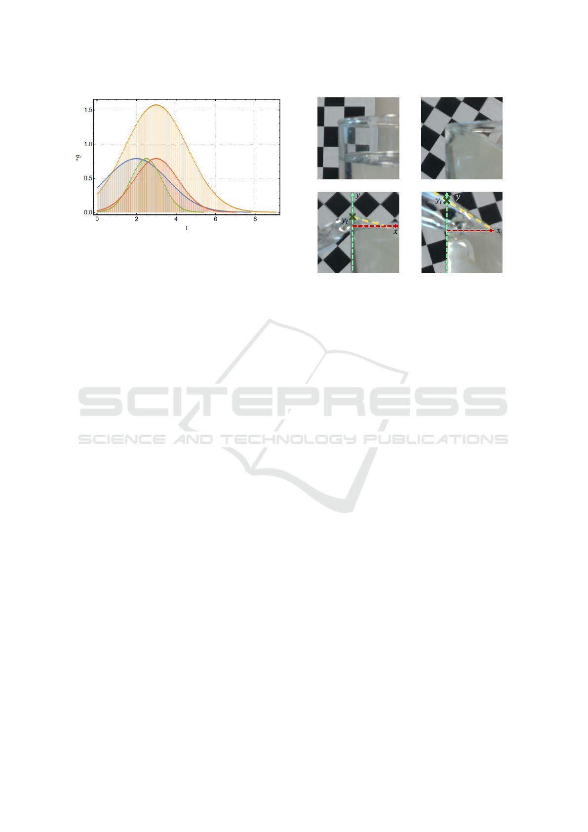
(a)
Figure 3: Different angle functions in time as applied to
the end effector. These curves have the property that they
increase the angles very slowly in order to generate waves
as few as possible.
A typical frame rate for storing images from the cam-
era and respective angle could be 30 fps.
In each experimental episode the resulting weight
as read on the scale w
E
is also stored, such that a data
set
E = (L
E
, w
E
)
is obtained for every experimental episode.
3.2 Controller Architecture
We propose a two stage setup. In a first stage the vol-
ume V
e
(estimated volume) of liquid leaving the con-
tainer as seen in a frame is calculated. OpenCV is
used to perform this preprocessing step.
As can be seen in figure 4 (c) and (d), the liquid
leaving the container has different forms depending
on the volume of the stream. The container always
has the same position in the image because the camera
is attached to the end effector. The chess pattern in
the background is used for demonstration purposes to
show the real angle of the end effector.
We propose a measure to describe the amount of
liquid leaving the container. Since the real flow of
liquid cannot be measured, a 2-dimensional geomet-
ric approach is chosen. The details are described in
section 3.3.1.
In the second stage, the estimated volume V
e
(as
described above) of the liquid in each frame is used
as an input for a policy network. The policy network
receives the estimated volume V
e
and a required goal
volume D to be filled up as an input. The output of
the policy network is a discretized relative angle ∆α,
where α is the angle of the actuator of the robot arm
which holds the container with the liquid. The control
in each time step is then applied as α ← α + ∆α.
(a) (b)
(c) (d)
Figure 4: Frames (a) to (d) show the pouring process from
the in-hand eye perspective. Pictures (c) and (d) show the
different forms of the pouring stream.
The total feedback control setup is then
Image → OpenCV → V
e
extracting information V
e
from the image, and then
using V
e
and D to receive ∆α
(V
e
, D) → MLP → ∆α
where MLP is a Multilayer Perceptron.
In each frame, the remaining volume D to be
poured into the recepient is reduced by the volume
V
e
of the triangle
D ← (D −V
e
) (2)
As the current volume in the receiving container
cannot be seen by the camera, the variable D serves
as an estimation of the remaining volume to be filled
up.
3.3 Training of Controller
The data collected from the experimental setup serves
as the training data for both components of the con-
troller: first, for estimating the liquid volume in each
frame as V
e
, and second, for training the angle con-
troller, which takes into account the frame’s volume
V
e
and the remaining goal volume D.
3.3.1 Volumes from Images
OpenCV is used to approximate the volume of the
poured liquid in each frame. This is done by calcu-
lating the 2d area of the triangle as shown in figure
4 (c) and (d). The y-axis aligns with the left side of
the container. The x-axis runs along the top edge of
Offline Feature-Based Reinforcement Learning with Preprocessed Image Inputs for Liquid Pouring Control
323

the glass. The yellow dotted line runs along the liq-
uid (intersection x-axis and y-axis). We denote with
V
e
the area of a triangle (yellow, red and green line)
in figure 4 (c) and (d). This way, a finite sequence of
values {V
1
e
,V
2
e
, . . . ,V
k
e
} is obtained during an experi-
mental episode. All of the values V
i
e
contribute to the
final output volume w
E
of an experimental episode.
The contribution of each V
i
e
depends on the number
of frames and frame rate applied. We define a nor-
malized contribution volume
ˆ
V
e
of each frame i as
ˆ
V
i
e
:= w
E
·
V
i
e
∑
k
j=1
V
j
e
Note that the normalized contribution volumes add up
to the total volume
k
∑
j=1
ˆ
V
i
e
= w
E
These normalized contribution volumes are used as an
input to the MLP described in the next section.
3.3.2 Offline RL for Angle Control
Policy. The second part of the algorithm consists of a
multi-layer perceptron (MLP) which works as a pol-
icy
π : O −→ {−10, . . . , 10}
(v
t
, v
t−1
, v
t−2
, d) 7→ ∆α
mapping the observation space O to a discretized rel-
ative angle ∆α of the end effector.
Observation Space. The observation space is de-
fined as
O := [0,V
max
]
3
× [−D
max
, D
max
] (3)
The observation space O ⊆ R
3
× R is 4-dimensional
(four real-valued input neurons) where V
max
in equa-
tion 3 is the maximal normalized contribution volume
as measured in phase 1 of the algorithm, and D
max
is
the maximal volume of the receiving container.
The first three arguments v
t
, v
t−1
, v
t−2
of the ob-
servation space are a sequence of the last three nor-
malized contribution volumes as described in section
3.3.1.
The second argument d of the observation space
stands for the volume which remains to be filled up.
Initially, if d = 0, the controller shall do nothing and
stay in the initial position. To activate the controller
and start the pouring process, d is set to the desired
goal volume
d ← V
G
(4)
to be poured into the receiving container. In each
frame d is reduced according to equation 2. If the
5.0
◦
3.5
◦
2.5
◦
1.5
◦
1.0
◦
0.7
◦
−5
◦
Figure 5: Distribution of the discretization of the relative
angles of the end effector. Relative angles close to zero are
discretized finer, relative angles close to −5
◦
and 5
◦
are dis-
cretized coarser.
remaining volume to be poured is eventually 0, the
controller shall rotate the joint back to its initial posi-
tion.
Since it may happen that the receiving container
receives too much liquid, also negative values for d
shall be allowed.
Action Space. The action space consists of the fol-
lowing 21 output neurons
{i|i = −10, ··· , 10}.
Each output neuron is mapped to a discretized rela-
tive angle α
i
according to figure 5. The relative angle
will then be applied to the angle α of the end effector
according to α ← α + α
i
.
Figure 5 shows the discretization of the relative
angles. Relative angles close to zero are discretized
finer to allow a control more precise.
Reward. A total reward function denoted as r is es-
tablished for every completed pouring process. It is
presumed that the pouring process concludes either
after a predefined number of frames or when all the
liquid has been emptied from container C. Let d rep-
resent the remaining volume that needs to be filled by
the end of the pouring process. When d reaches 0, it
signifies that the target volume V
G
has been precisely
achieved.
Define r(d) as
r(d) := e
−(δ·d
2
)
(5)
where δ < 1 is typically a small number which defines
the width of the reward function around the desired
goal value. Note that a reward is given only at the end
of the sequence.
Training. With the defined observation space, action
space, and reward structure, a feedback controller can
be trained using reinforcement learning techniques.
In this scenario, only offline data, as outlined in sec-
tion 3.1, is accessible, and direct interaction between
ICINCO 2023 - 20th International Conference on Informatics in Control, Automation and Robotics
324

the agent and the physical system is not possible.
Consequently, traditional exploration methods are not
viable. Our proposed approach involves employing a
policy gradient method based on Monte-Carlo policy
gradient techniques, akin to the REINFORCE method
as described in (Williams, 1992).
We enrich the sequences obtained from the exper-
iments with the physical system described in section
3.1 to generate training sequences.
Training Data Generation. We propose the fol-
lowing method to generate a sufficiently rich set of
training data. A sequence from a single experimen-
tal episode E may be used as multiple episodes for
training. Given an experimental episode
L
E
= {(Image
i
, α(i)) : i}
together with a final volume w
E
. Then training se-
quences are generated as follows:
1. From each Image
i
calculate the normalized con-
tribution volume of the liquid pouring from the
container as described in section 3.3.1 to obain a
sequence {
ˆ
V
1
e
, . . . ,
ˆ
V
k
e
}.
2. For each i = 1, 2, . .. , k, calculate the relative an-
gles as ∆α(i) := α(i) − α(i − 1). Apply the dis-
cretization of the relative angles as explained in
figure 5 to obtain a sequence of values ∆α
i
∈
{−10, . . . , 10}
3. Choose an initial goal volume V
G
for this experi-
mental episode according to the following rule:
V
G
(κ) := κ · w
E
, κ = 0.5, . . ., 1.5. (6)
For each κ a different goal volume is created.
Therefore, for each κ a different training sequence
is created. E.g. for κ = 1.0, the goal volume
V
G
(κ) is equal to the volume w
E
from this exper-
imental episode. Therefore a perfect pouring pro-
cess is obtained which meets exactly the goal vol-
ume V
G
. For κ = 0.5, the goal volume V
G
=
w
E
2
.
This creates a training sequence, where too much
liquid is poured into the goal container:
w
E
2
is de-
sired, but w
E
is obtained. For κ = 1.5 we obtain
a training sequence in which too little liquid is
poured into the receiving container.
4. Calculate the sequence d
i
of remaining liquid vol-
ume to be poured. For i = 0 choose d
0
= V
G
(κ)
from equation 6 and calculate
d
i+1
:= d
i
−
ˆ
V
i
e
to obtain a sequence {d
0
, d
1
, ·· · , d
k
}.
5. Calculate the reward of the sequence using defini-
tion 5
R
E
:= r(d
k
)
6. To create a baseline, take all total rewards R
E,i
from all experimental episodes and calculate the
mean R
E
and the variance σ
E
to receive normal-
ized rewards
ˆ
R
E,i
:=
R
E
− R
E
σ
E
(7)
7. For every state ω
i
and action ∆α
i
from the exper-
imental episodes, take the one-hot encoded action
I
i
= (0, . . . , 0, 1, 0, . .. , 0) ∈ {0, 1}
21
, where the 1
stands at the position which represents the action
taken in the state ω
i
in the experimental episode.
8. Apply a softmax function to the output of the
multi-layer perceptron to receive a probability dis-
tribution p
i
for the 21 possible actions. Train the
artificial neural network in the respective state ω
i
,
applying
ˆ
R
E,i
· I
i
, i.e. set the desired output Y (la-
bel) of the artificial neural network to
Y := (1 − λ ·
ˆ
R
E,i
) · p
i
+ λ ·
ˆ
R
E,i
· I
i
(8)
where λ ∈ (0, 1) is a learning factor. Use the cat-
egorical cross-entropy loss function to train the
neural network.
Observe, that equation 8 describes a function
{−10, . . . , 10} → R in which all values add up to
1, and negative values may occur. This is due to
p
i
and I
i
being probability distributions, and
ˆ
R
E,i
may be negative.
The training of the multi-layer perceptron is done in
adequate batches with samples taken randomly from
the experimental episodes.
Observe, that REINFORCE is actually an on-
policy method. To use REINFORCE with offline
data, usually a correction using importance sampling
has to be made to account for the distributional shift,
because the sampling data is taken from a different
distribution as the one to be corrected for, see e.g.
(Liu et al., 2019), (Levine et al., 2020), (Kallus and
Uehara, 2020).
In the case described in this paper, the samples
from the experimental episodes do not correspond to
a particular policy. Therefore corrections cannot be
made or are difficult to introduce. The method is ex-
pected to work similar to cross-entropy methods, see
e.g. (Kroese et al., 2005).
4 EXPERIMENTAL RESULTS
Experiments were conducted using a simple simula-
tion for pouring liquids. The general properties and
functioning of the algorithm could thus be proven.
A simulation has been implemented which gener-
ates volumes V (corresponding to V
e
as described in
Offline Feature-Based Reinforcement Learning with Preprocessed Image Inputs for Liquid Pouring Control
325

section 3) of triangles depending linearly on the angle
α and the remaining volume in the container.
A multi-layer perceptron with two hidden layers
and 2000 parameters is trained. To simplify the ex-
periments, only two actions are used: ∆α ∈ {−1, 1}.
A single experimental episode of the robot arm is
used as an offline training sequence, creating multiple
training sequences by applying random goal volumes
according to equation 6.
Experiments show a fast convergence. The result-
ing policy network pours liquid within the simulation
matching an arbitrary given goal volume.
5 CONCLUSION
A method has been outlined for constructing a con-
troller tasked with pouring a specified quantity of liq-
uid into a receiving container.
The approach comprises two primary steps: first, a
preprocessing phase that extracts relevant image fea-
tures, followed by the implementation of a policy net-
work. Importantly, the policy network operates with
a low input dimension, as image preprocessing is ap-
plied using a separate image processing tool.
In addition, only ground truth data measured from
the real laboratory setup is used. Therefore, no simu-
lation of the setup is required to train the policy net-
work. The policy network is trained in an offline man-
ner using the data from the laboratory setup.
A valuable aspect of the proposed approach is its
capacity to derive multiple training sequences from a
single experimental sequence.
The method presented in this paper exhibits ro-
bustness in handling variations in the initial volumes
within the source container, achieved through control
of relative pouring angles. Moreover, the method ex-
clusively measures the liquid exiting the source con-
tainer, enabling its applicability in scenarios where
the liquid within the target container is not visible or
measurable, such as when watering plants.
The method has been implemented within a pour-
ing liquid simulation and shows fast convergence and
independence of goal volumes. Next, the data from
the physical system will be included to generate a
controller for the UR5 robot arm.
REFERENCES
Arora, S. and Doshi, P. (2021). A survey of inverse
reinforcement learning: Challenges, methods and
progress. Artificial Intelligence, 297:103500.
Cobo, M., Heredia, I., Aguilar, F., Lloret Iglesias, L.,
Garc
´
ıa, D., Bartolom
´
e, B., Moreno-Arribas, M. V.,
Yuste, S., P
´
erez-Matute, P., and Motilva, M.-J. (2022).
Artificial intelligence to estimate wine volume from
single-view images. Heliyon, 8(9):e10557.
Kallus, N. and Uehara, M. (2020). Statistically efficient off-
policy policy gradients.
Kroese, D., Mannor, S., and Rubinstein, R. (2005). A tu-
torial on the cross-entropy method. Annals of Opera-
tions Research, 134.
Levine, S., Kumar, A., Tucker, G., and Fu, J. (2020). Offline
reinforcement learning: Tutorial, review, and perspec-
tives on open problems. CoRR, abs/2005.01643.
Liu, Y., Swaminathan, A., Agarwal, A., and Brunskill, E.
(2019). Off-policy policy gradient with state distribu-
tion correction.
Liu, Z., Liu, F., Zeng, Q., Yin, X., and Yang, Y. (2023). Es-
timation of drinking water volume of laboratory ani-
mals based on image processing. Scientific Reports,
13.
Moradi, H., Masouleh, M. T., and Moshiri, B. (2021).
Robots learn visual pouring task using deep reinforce-
ment learning with minimal human effort. pages 504–
510. Institute of Electrical and Electronics Engineers
Inc.
Pareigis, S. and Maaß, F. L. (2023). Improved Robust Neu-
ral Network for Sim2Real Gap in System Dynamics
for End-To-End Autonomous Driving. LNEE Series
published by Springer, to appear.
Schenck, C. and Fox, D. (2017). Visual closed-loop control
for pouring liquids. In 2017 IEEE International Con-
ference on Robotics and Automation (ICRA), pages
2629–2636.
Sutton, R. S. and Barto, A. G. (2018). Reinforcement Learn-
ing: An Introduction. The MIT Press, second edition.
Tamosiunaite, M., Nemec, B., Ude, A., and W
¨
org
¨
otter, F.
(2011). Learning to pour with a robot arm combining
goal and shape learning for dynamic movement prim-
itives. Robotics and Autonomous Systems, 59:910–
922.
Williams, R. J. (1992). Simple statistical gradient-following
algorithms for connectionist reinforcement learning.
Mach. Learn., 8(3–4):229–256.
Zhao, W., Pe
˜
na Queralta, J., and Westerlund, T. (2020).
Sim-to-Real Transfer in Deep Reinforcement Learn-
ing for Robotics: a Survey. arXiv e-prints, page
arXiv:2009.13303.
ICINCO 2023 - 20th International Conference on Informatics in Control, Automation and Robotics
326