Preliminary Results on Controllability of Serial Robot-Manipulators in

Singular Conﬁgurations

Mir Mamunuzzaman and J

org Mareczek

Faculty of Electrical and Industrial Engineering, Landshut University of Applied Sciences, 84036 Landshut, Germany

Keywords:

Singularity, Non-Linear Controllability, Jacobian, Robot Motion Planning.

Abstract:

We develop a standard system representation and analyse controllability properties for velocity kinematics

of robot-manipulators located on singularities. These are positions where the Jacobian loses rank. Since its

column vectors span the set of admissible workspace velocity directions, it is still a widespread misunder-

standing that some directions would be locked on singularities and thus had to be bypassed as far as possible.

We will show that this does not generally hold: On some types of singularities, the kinematic shows local

redundancy, which can be used to generate paths crossing the singularity in any desired workspace velocity

direction. To further analyse controllability properties, we develop an SVD-based method to represent the

Jacobian-based velocity kinematics in standard system description of control theory without the need for in-

verse kinematics (IK). In many cases, IK do not offer a unique solution on singularities and, therefore, cannot

be used. Furthermore, we present a modiﬁcation of the SVD-based method for which the analytical calcula-

tion effort is feasible. The resulting system description has the advantage of being a simple decoupled set of

single-integrators where the system states are divided into one set describing admissible workspace motions

and a second set describing possible internal motions, also called nullspace motion. Based on this standard

system representation, we determine local controllability and local accessibility for two different types of sin-

gularities. Finally, we illustrate our methods by means of a simple 3-DoF SCARA-type manipulator.

1 INTRODUCTION

Ongoing industrial transformation includes more net-

worked, automated and intelligent manufacturing

lines, (Kuo et al., 2017), (Mazzanti et al., 2019), (Na-

havandi, 2019). This leads to an increasing de-

gree of autonomy in industrial automation planning.

One emerging technology towards this direction is

computer-aided manufacturing (CAM), which aims to

connect CAD directly with a CNC tooling machine.

Beyond that, more and more industrial robots (in the

following denoted as manipulators) are used for tool-

ing. They offer the advantage of high dexterity and

a large workspace. Prominent examples are additive

manufacturing with large-scale 3D-printing, cladding

or buildup welding, cover manipulation or human-

robot collaboration.

These new manufacturing processes are charac-

terized by paths that are either very long or non-

predictable and are changed very often. This can also

be observed in many other ﬁelds of applications like

telesurgery, emergency manipulation inside nuclear

reactor cells and explosive ordnance disposal.

Clearly, these types of paths cannot be imple-

mented anymore by classical manual teaching or pro-

gramming; the corresponding work effort would be

excessive. In contrast to that, modern path plan-

ning requires the calculation of adequate joint paths

(jointspace) from given, desired paths of the end-

effector (workspace); the corresponding mapping

from workspace to jointspace is denoted as inverse

kinematics (IK). Problems arise from the fact that a

method to solve IK analytically is only known for a

very restricted type of kinematics fulﬁlling Pieper’s

requirements. Moreover, IK for six or more joints suf-

fer from a high computational complexity.

In addition to joint positions, path-tracking con-

trol also requires joint velocities as feed-forward con-

trol input. These velocities are calculated by means

of the inverse of the Jacobian matrix (in the following

denoted as Jacobian) of the direct kinematics.

Unfortunately, the rank of the Jacobian typically

depends on joint positions, and there exist positions

where it loses rank, so-called singularities. It is well

known that approaching such a singularity turns into

excessively large joint speeds unless the commanded

Mamunuzzaman, M. and Mareczek, J.

Preliminary Results on Controllability of Serial Robot-Manipulators in Singular Conﬁgurations.

DOI: 10.5220/0012238000003543

In Proceedings of the 20th International Conference on Informatics in Control, Automation and Robotics (ICINCO 2023) - Volume 1, pages 327-334

ISBN: 978-989-758-670-5; ISSN: 2184-2809

327

end-effector speed points into a special set of ad-

missible directions. Although this problem has been

known from the very beginning of robotics, singular-

ities still suffer from little research interest. In fact,

it is the general view of many roboticists that singu-

larities impose an unsolvable problem and are thus to

be bypassed as far as possible. This is also the basic

idea behind all existing control methods, for exam-

ple, damped least-square control (DLSC), (Wampler,

1986) or related methods like Non-Redundancy Sin-

gularity Avoidance (NRSA), (Huang et al., 2016),

Singularity Avoidance System (SAS), (Raineri and

Bianco, 2017), Partially Decoupling and Lineariz-

ing Control, (PDLC), (Mareczek, 2020). These ap-

proaches all lead to restrictions in tracking perfor-

mance within close vicinities of singularities (called

singular regions); these restrictions are not tolerable

in many applications.

However, singularities may also offer advantages:

Here, a manipulator can show local redundancy. Fur-

thermore, maximum forces and torques exerted by

the end-effector on the environment depend only on

break limits of mechanics rather than on actuator lim-

itations. For these reasons, a path planning method

together with an appropriate control which does not

have to avoid singularities is desirable. In fact, it is

not necessary to avoid all kinds of singularities: As

we will show by an example, there always exists a

smooth path crossing one type of singularity in any

predeﬁned workspace direction. This is possible by

taking advantage of kinematic redundancy available

locally on that type of singularity.

Questions concerning admissible directions into

which the system states may evolve can be charac-

terized by its controllability properties. Therefore,

this paper focuses on a standard system description of

control theory for Jacobian-based velocity kinemat-

ics. Based on that, we present preliminary results

towards the characterization of singularities with re-

spect to controllability properties.

Actually, no such classiﬁcation of singularities

can be found in literature. Instead, common ways

to classify singularities are: internal or boundary

type, see for example (Spong et al., 2020). In (Ki-

effer, 1994) isolated and bifurcation type of singular-

ities are deﬁned by a differential geometric approach

characterising the curve geometry of achievable paths

in workspace. This approach uses the solution for

IK, entailing its above-mentioned problems. Interest-

ingly, the author suggests to “make use of kinematic

singularities, rather than simply negotiate past them”.

In (Nielsen et al., 1991), controllability has been

investigated with respect to the standard rigid body

model from mechanics. Hence, this system descrip-

tion is very complicated. Today’s drive systems (mo-

tors with gears) are fast enough to operate in velocity

rather than torque mode. Therefore, velocity kinemat-

ics are primarily used for motion control. However,

the authors also concluded: “One may consider [other

possibilities for controller design] instead of just giv-

ing up and saying that control in certain directions is

impossible at singularities”.

From the point of view of nonlinear control the-

ory, the Jacobian-based velocity kinematics represent

a nonlinear driftless system with the Jacobian column

vectors as control vector ﬁelds. However, the latter

depends on the time-integral of the control input vari-

ables. IK can solve this problem, but not on types

of singularities where IK don’t offer a unique solu-

tion. Therefore, we present a method to transform

the Jacobian-based velocity kinematics into a stan-

dard system description without IK, thus being ap-

plicable and valid on singularities, also. Further ad-

vantages are: Decoupling of dynamics for admissi-

ble workspace motion and possible internal dynam-

ics (nullspace motion). Thus, the nature of variable

structure shows clearly by the variable number of sys-

tem states describing admissible workspace motion.

Moreover, this leads to a natural and easy way to in-

vestigate and classify internal dynamics. Last but not

least, the new system appears as a decoupled set of

single integrators, which strongly simpliﬁes further

system analysis and proofs.

We organize our paper as follows: First, we de-

velop a method based on SVD to rewrite the velocity

kinematics in the standard description of control the-

ory without the need for IK. Then, in section 3, we

present decoupling of the dynamics. In Section 4, we

prove that for this sample kinematic, there always ex-

ists a smooth path crossing on type of singularities.

Finally, in section 5, we apply the proposed method to

a simple SCARA-type kinematic and conclude with

some preliminary results on controllability.

2 PROBLEM FORMULATION

In this section, we outline the control problem of

robot-manipulators on singularities. To do this, let’s

ﬁrst review the kinematics of serial robotic manipula-

tors. The reader is referred to standard textbooks for

more details on robot kinematics.

We start by recalling the distinction between

redundant and non-redundant robot-manipulators.

There are various ways to deﬁne redundancy (Conkur

and Buckingham, 1997). In this work, we solely take

kinematic redundancy into account. The workspace

for robot-manipulators typically describes the carte-

ICINCO 2023 - 20th International Conference on Informatics in Control, Automation and Robotics

328

sian position (e.g., x, y, z) and/or orientation (e.g.,

Euler-angles α, β, γ) of the robot’s end-effector. For

robot-manipulators, the variables that deﬁne the

conﬁguration comprise the jointspace. When the

workspace and jointspace dimension are the same

a robot-manipulator is said to be non-redundant. On

the other hand, the manipulator is considered redun-

dant when the workspace dimension is greater than

the jointspace dimension.

Consider a non-redundant serial-link robot ma-

nipulator with n rigid links connected by revolute

or prismatic joints. Deﬁning n joint variables by

q =



··· q



∈ Q ⊂ R

, which is also

referred to a conﬁguration, and n workspace coordi-

nates by η

η =



··· η



∈P ⊂R

, the for-

ward kinematics are expressed as

η = f(q), (1)

with a non-linear, continuous and differentiable direct

mapping f : Q 7→P . The IK problem is to compute the

inverse mapping, f

−1

, that gives us joint variables for

a given ﬁxed end-effector’s position and orientation.

There is a countable set of solutions possible:

−1

: (η

η, κ) 7→ q, κ ∈ {1, ··· , k} (2)

with k as the number of possible conﬁgurations.

Moreover, the solutions of IK may be inﬁnite (hence

an uncountable set of solutions), or no solution at all

may exist.

Differentiating equation (1) with respect to time

yields

η =

f(q(t)) =

∂f(q)

∂q

q =

J(q)

q =

∑

i=1

(q) ˙q

, (3)

where

J(q) =



(q) j

(q) ··· j

(q)



∈ R

n×n

the conﬁguration dependant Jacobian of f(q).

In this work, we deﬁne a conﬁguration as singu-

lar when the Jacobian loses one or more ranks, hence

if det(

J) = 0. This leads to the severe restriction that

the robot’s end-effector can no longer move in cer-

tain directions. To investigate this in more detail, we

split the space of motion of the end-effector into two

subspaces: regular space, which contains admissible

directions, and singular space, which contains locked

directions. The singular space must be an orthonor-

mal complement of the range of

J, which establishes

the regular space.

However, it is still possible to move in the direc-

tion of singular space in some cases, as we will show

later. To ﬁnd out under which conditions this is pos-

sible, we consider velocity kinematics (3) as a control

We assume the workspace and the jointspace both to

be expressed in minimal coordinates.

system and investigate its controllability properties on

the singular subspace. First, let’s recall the standard

general nonlinear system representation:

x = g

(x) +

∑

i=1

(x)u

, (4)

where x ∈ R

contains the system-states, u =



··· u



∈ R

are the control-input variables,

and g

, i ∈ {0,··· , n} are smooth vector ﬁelds deﬁn-

ing the unforced (g

: drift) and forced (g

, g

,···:

control) motions. Comparing (3) with standard model

(4) yields g

= 0 (driftless system), joint angle veloc-

ities as control-inputs u =

q, workspace variables as

system-states x = η

η, and columns of

J(q) as control

vector ﬁelds. The latter, however, explicitly depend

on joint variables q rather than on system-states η

η.

One approach to eliminate the dependency of q is by

substituting the IK (2):

η =

J(f

−1

(η

η,κ ))

The IK, nonetheless, are only known for a few ba-

sic kinematics. Furthermore, most kinematics do not

have a unique solution for the IK on a singularity. As

a result, this strategy does not apply to most manipu-

lators. Instead, we prefer a system model, see section

3, that does not require the knowledge of IK.

Additionally, the primary instrument for analysing

controllability of a non-linear system, Lie brackets

from differential geometry, cannot be used since nec-

essary smoothness assumptions are not met on singu-

larities. For system (3), we can see this issue mathe-

matically. The Lie brackets of any two vector ﬁelds

can be expressed by

] =

∂j

∂η

−

∂j

∂η

It is apparent that, on singularities,

∂j

∂η

is not deﬁned

in all workspace directions ∂η

η. Therefore, the differ-

ential geometric approach to controllability analysis

on singularities cannot be applied.

3 SYSTEM REPRESENTATION

As starting point for a state-space formulation of the

system on singularities, in the system description, in

addition to the dynamics for the workspace variables

η, we also take into account the dynamics for joint

space variables q:

η =

J(q) u

q = u

(5)

This seems to increase the system’s total number of

state variables to 2n. The number of state variables,

Preliminary Results on Controllability of Serial Robot-Manipulators in Singular Conﬁgurations

329

however, remains n since the forward kinematics con-

strains the joint space variables to the workspace vari-

ables.

It has already been stated that the Jacobian loses

ranks on singular conﬁgurations. We deﬁne a set that

includes all singular conﬁgurations by

Q = {q |det(

J(q)) = 0}. (6)

Elements of the above set are denoted as q

∗

. Let, on

∗

∈Q, the Jacobian loses r ranks, i.e., rank(

J(q

∗

)) =

n −r. This conﬁguration is also called a singular con-

ﬁguration of codimension r.

To better understand possible motions on singular-

ities, we decouple the system-states into two groups:

One spanning the regular space, the other one span-

ning the singular space. This can be performed by

singular value decomposition (SVD). An eigenvalue

decomposition (EVD) could also be applied as alter-

native to SVD in case of a quadratic Jacobian. How-

ever, unlike EVD, SVD can also be used to address

the more general case of redundant manipulators (i.e.,

non-square Jacobian).

Let us consider a singularity of codimension r.

Here, the SVD of the manipulator Jacobian

J(q

∗

) can

be decomposed into

J(q

∗

) =

U(q

∗

)

Σ(q

∗

)

∗

), (7)

where columns u

U and v

V for i ∈ {1, ··· , n}

form an orthonormal basis of R

, and singular values

∗

, i ∈ {1,···, n} with the r smallest singular values

equal to zero form the diagonal matrix

Σ(q

∗

) ∈ R

n×n

Without loss of generality we may assume that all

vanishing singular values are gathered at the end, i.e.,

Σ(q

∗

) = diag{σ

∗

,··· , σ

∗

n−r

, 0, ··· , 0}. Denoting the

left and right singular matrix on a singular conﬁgura-

tion with

∗

U(q

∗

) and

∗

V (q

∗

) and the diag-

onal matrix by

∗

Σ(q

∗

) = diag{

∗

, 0, ··· , 0}, the

SVD of

J(q

∗

) can be expressed as

∗

∗T

, (8)

where

∗

is a diagonal matrix comprised of all non-

zero singular values of the Jacobian. We now develop

a state-space representation for the velocity kinemat-

ics using SVD of the Jacobian on singular conﬁgura-

tions:

Proposition 3.1. Assume velocity kinematics (5) are

on a singular conﬁguration. We introduce a virtual

control ζ

ζ =



··· ζ



. Then by deﬁning n new

system states z =



··· z



, it’s always possible

to rewrite system representation (5) in the following

decoupled form:

z = ζ

q = h(q)ζ

ζ,

(9)

with h(q) as a virtual control function possibly non-

linearly relates the virtual and the actual control vari-

ables.

Proof. The assumption that velocity kinematics (5)

are on a singular conﬁguration implies rank deﬁ-

ciency of the Jacobian. Let us consider a singular-

ity of codimension r. The left singular matrix

∗

can be decomposed as

∗



∗



with

∗



∗

··· u

∗

n−r



∈R

n×n−r

that spans the range space

∗

, i.e., R (

∗

) and

∗



∗

n−r+1

··· u

∗



∈

n×r

that spans the singular space of

∗

. Similarly,

the right singular matrix

∗

can also be decomposed

∗



∗



with

∗



∗

··· v

∗

n−r



∈

n×n−r

, and

∗



∗

n−r+1

··· v

∗



∈ R

n×r

that

spans the null space of

∗

, i.e., N (

∗

We deﬁne (n −r) new system states so that

(˙z

··· ˙z

n−r

)

∗T

η. (10)

Using velocity kinematics and performing SVD on

the Jacobian, from (10), it follows:

(˙z

··· ˙z

n−r

)

∗T

∗

∗T

q =

∗

∗T

(11)

Next, using the non-zero singular values of the Jaco-

bian, we deﬁne a diagonal matrix as follows:

∗

S(q

∗

) = diag{σ

∗

,··· , σ

∗

n−r

, 1, ··· , 1}.

Note that the last r elements of the above diagonal ma-

trix are set to a constant, non-zero value just to make it

invertible. For convenience we chose number 1. The

inverse, hence, exists by construction:

∗−1

= diag{σ

∗−1

,··· ,σ

∗

n−r

−1

, 1, ··· , 1}.

With

∗−1

, we deﬁne virtual control variables ζ

ζ =

(ζ

··· ζ

)

q = h(q

∗

)ζ

ζ =

∗

∗−1

ζ (12)

In this case, (ζ

··· ζ

n−r

)

are to control in non-

singular directions, while (ζ

n−r+1

··· ζ

)

are to con-

trol potentially existing internal dynamics in the

singular direction. Inserting (12) in (11) yields

∗

∗T

∗

∗−1

ζ =



··· ζ

n−r



and, thus, we

obtain a set of single-integrator systems:

˙z

= ζ

, i ∈{1, ··· , n −r}. (13)

Given (13), it is evident that the last r elements of the

virtual control, i.e., (ζ

n−r+1

··· ζ

)

are not included

in the system description (as desired), but are included

in (12) to determine

q. If one resolves (12) for ζ

ζ, the

results are:

ζ =

∗

∗T

q ⇒ζ

(

∗

∗T

q, i ∈ {1, ··· , n −r}

∗T

q, i ∈ {n −r + 1, ··· , n}

ICINCO 2023 - 20th International Conference on Informatics in Control, Automation and Robotics

330

Therefore, the last r rows deﬁne the dynamics in sin-

gular space. It completes the total dynamics of the

system, including singular and non-singular direc-

tions. To get a standard form of the dynamics in sin-

gular space, a locally reversible coordinate transfor-

mation q ∈ R

7→ z

∈ R, for i = {n −r + 1, ··· , n}

is deﬁned in such a way that it satisﬁes the following

time derivative:

˙z

= v

∗T

(q)

q. (14)

This new set of variables (z

n−r

··· z

)

contains the

state variables describing the dynamics in singular di-

rections. In summary, the complete state space repre-

sentation thus follows from (13) and (14) to

z = ζ

ζ, with

q = h(q)ζ

ζ = V

∗

∗−1

ζ.

Remark: In comparison to (5), state-space rep-

resentation (9) has the advantage of totally decou-

pling workspace dynamics (described by z) from joint

space dynamics. Another signiﬁcant advantage is

that the workspace dynamics are separated into a

non-singular range (z

··· z

n−r

)

and a singular range

n−r+1

··· z

)

3.1 Alternative Decomposition of

In the previous section, we observe that for rewrit-

ing the system dynamics, we need to compute

∗

and

∗

on singular conﬁgurations. With a large Ja-

cobian, however, an analytical expression to perform

SVD is highly complex. Hence, we propose an alter-

native and less complex method to SVD:

Proposition 3.2. Assume velocity kinematics (5) are

on a singular conﬁguration. Consider virtual control

ζ = (ζ

··· ζ

)

, deﬁned by:

q =

∗

ζ =

K(q

∗

)ζ

ζ =



∗

··· k

∗



ζ, with matrix

∗

∈ R

n×n

. Con-

struct an orthonormal matrix

∗

W (q

∗

) = [w

∗

···w

∗

n−r

∗

···n

∗

] ∈ R

n×n

such that its ﬁrst (n − r) columns {w

∗

···w

∗

n−r

}

span R (

∗

), and the last r columns {n

∗

···n

∗

} span

N (

∗T

). If n new system-states

z = (˙z

··· ˙z

)

satisfy

z =

∗T

η, then it is always possible to construct a

∗

that satisﬁes the decoupled state-space representation

in (9) with

q =

∗

ζ.

Proof. Consider (5) on a singular conﬁguration of

codimension r. According to the fundamental theo-

rem of linear algebra, the following holds:

1. dim(R (

∗

)) = n −r and dim(N (

∗T

)) = r

2. N (

∗T

) is the orthogonal complement to R (

∗

)

By construction,

∗

is an orthogonal matrix, with its

ﬁrst n −r columns describing non-singular directions

and the last r columns describing singular directions.

Next, we consider n new system-states such that

the ﬁrst (n −r) states (z

··· z

n−r

)

describe the non-

singular dynamics and the last r states (z

n−r+1

··· z

)

describe the singular dynamics, and assume, they sat-

isfy the following relation:

z =

∗T

(3)

∗T

∗

q. (15)

Since the last r columns span the space N (

∗T

it follows that all elements of the last r rows of

∗T

∗

become zero, so that ˙z

= 0, i ∈ {n −r +

1, ··· , n}. Next we deﬁne virtual control variables ζ

q =



∗

··· k

∗



ζ with {k

∗

n−r+1

,··· ,k

∗

}∈

N (

∗

). From (15) we further obtain

z =

∗T

∗

ζ.

We deﬁne a matrix

a×b

∈ R

a×b

which comprises

an identity matrix I

min{a,b}

and the rest of the elements

are zeros. Since the last r rows of

∗T

∗

vanish, we

can reduce it to an n −r dimension identity matrix i.e.,

n−r×n

∗T

∗



∗

n−r+1

··· k

∗



n−r×n

In order to achieve a decoupled dynamic in



n−r+1

··· z



, one can arbitrarily choose k

i j

= 0

for i ∈ {n −r + 1,··· , n} and j ∈ {1, ··· , n −r} in

the above underdetermined system. The remaining

∗



··· k

i(n−r)



results in a unique soluton:



∗

··· k

∗

n−r





n−r×n

∗T

∗

n×n−r



−1

Finally, along with the last r columns of

∗

, the fol-

lowing relation

z =

∗T

∗

ζ = diag{1, .. ., 1,0, .. ., 0}ζ

ζ (16)

gives the desired state-space representation in single

integrator form:



˙z

··· ˙z

n−r

˙q

n−r+1

··· ˙q



= ζ

ζ.

Remark: Expression (16) is similar to SVD

∗T

∗

= diag{σ

∗

, ··· , σ

∗

n−r

, 0, ··· , 0} with

two matrices

∗T

and

∗

that are analogous to the left

and right singular matrices

∗T

and

∗

. The differ-

ence is that a normalized matrix is considered while

constructing

∗T

and the orthonormality criterion in

∗

is lost while constructing

∗

4 CONTROLLABILITY

In this section, we will investigate the controllability

of serial robotic manipulators with the above formu-

lated feed-forward control law (12) on different sin-

gular conﬁgurations. It is already stated in section

Preliminary Results on Controllability of Serial Robot-Manipulators in Singular Conﬁgurations

331

2 that differential geometric techniques, commonly

used in the analysis of controllability and accessibility

of nonlinear systems, are inapplicable due to the lack

of smoothness around the singularity. Before going

further, we ﬁrst demonstrate that

Proposition 4.1. The proposed control law (12) is

continuous on an open-ball vicinity of singular con-

ﬁgurations.

Proof. Outside the singular conﬁguration, the joint

angle trajectory is always well-deﬁned by

q =

−1

(η

η, κ ))

η, since the inverse kinematics have

a unique solution, and the Jacobian has full rank. On

singularity, control law (12) gives the unique solution

for the inverse of the velocity dynamics. This leaves

only the case when we are in a vicinity of the singu-

larity, i.e., q → q

∗

. For continuity, it is sufﬁcient to

show that the following relation holds:

lim

q→q

∗

V (q)

−1

(q)ζ

ζ = q

∗

. (17)

If this does not hold, then there exists a ε

ε ∈ R

̸= 0

such that

lim

q→q

∗

V (q)

−1

(q)ζ

ζ −q

∗

= ε

ε. (18)

Then left multiplication with (

∗

∗T

) leads to

lim

q→q

∗

(

∗

∗T

V (q)

−1

(q)ζ

ζ) −

∗

∗T

∗

∗T

ε.

The left side of this equation further details to:

lim

q→q

∗

(

∗

∗T

V (q)

−1

(q)ζ

ζ) −

∗

∗T

∗

∗T

∗

lim

q→q

∗

(

−1

(q)ζ

ζ) −

∗

∗T

∗

lim

q→q

∗

(

−1

(q)ζ

ζ) −

∗

∗T

∗

∗−1

∗

−ζ

∗

= diag{σ

∗

∗−1

,··· ,σ

∗

n−r

∗

n−r

−1

,1, ··· , 1}ζ

∗

−ζ

∗

= 0

Since the right-hand side of (18) certainly does not

vanish, this contradicts the above assumption; there-

fore, (17) must be valid. Hence, by construction, the

feed-forward control law is continuous.

At this point, we discuss control strategies of

robot-manipulators on singularities. The system rep-

resentation is ﬁrst formulated close to singular conﬁg-

urations, as shown in section 3. This provides us with

n −r control input variables for admissible motion in

workspace and r control input variables for null space

motion in singular space. Depending on the nature of

the singularity, the null space motion can then be used

to escape it.

Singularities of redundant manipulators, based on

the presence of internal motion (also known as self-

motion), are classiﬁed into two categories, see, e.g.,

(Chang and Khatib, 1995), (Oetomo and Ang, 2009).

Internal motion changes joint conﬁguration with con-

stant end-effector pose. Type-1 singularities, where

internal motion caused by null space motion changes

the singular direction, and Type-2 singularities, where

the null space motion doesn’t provide any internal

motion – moving in any direction is not possible.

Similarly, for non-redundant manipulators, based

on the presence of internal motion, we classify sin-

gularities in Type-1 and Type-2 singularities since

non-redundant manipulators show local redundancy

on some singularities. To begin, it is crucial to deter-

mine which singularities provides internal motion.

In (6), a set Q was deﬁned that contains all singu-

lar conﬁgurations. Consider, P to be an open subset

of Q i.e., P ⊆ Q. Let’s deﬁne a function on P as

P 7→ R : Φ(q) = det(

J). (19)

Then, P is time-invariant if

Φ(q) = 0 holds for all q ∈

P. In other words, internal motion is possible due to

null space motion in the open subset P. The following

lemma gives us a sufﬁcient condition for the existence

of internal motion on singularities in (9):

Lemma 4.2. A sufﬁcient condition for existence of

internal motion is

∂Φ(q)

/∂q

K(q)[n −r +1 : n] = 0 for

all q ∈ P.

Proof. Differentiating (19) yields

Φ =

∂Φ(q)

∂q

∂det(

J(q))

∂q

∗

ζ.

By deﬁnition of internal motion

Φ must vanish:

∂Φ(q)

/∂q

∗

ζ = 0. On the singular surface P, ζ

··· = ζ

n−r

= 0 so that for all ζ

n−r+1

,··· ,ζ

∈ R

∂Φ(q)

/∂q



∗

n−r+1

··· k

∗



n−r+1

···ζ



= 0

⇐⇒

∂Φ(q)

/∂q



∗

n−r+1

··· k

∗



= 0

5 NUMERICAL EXAMPLE

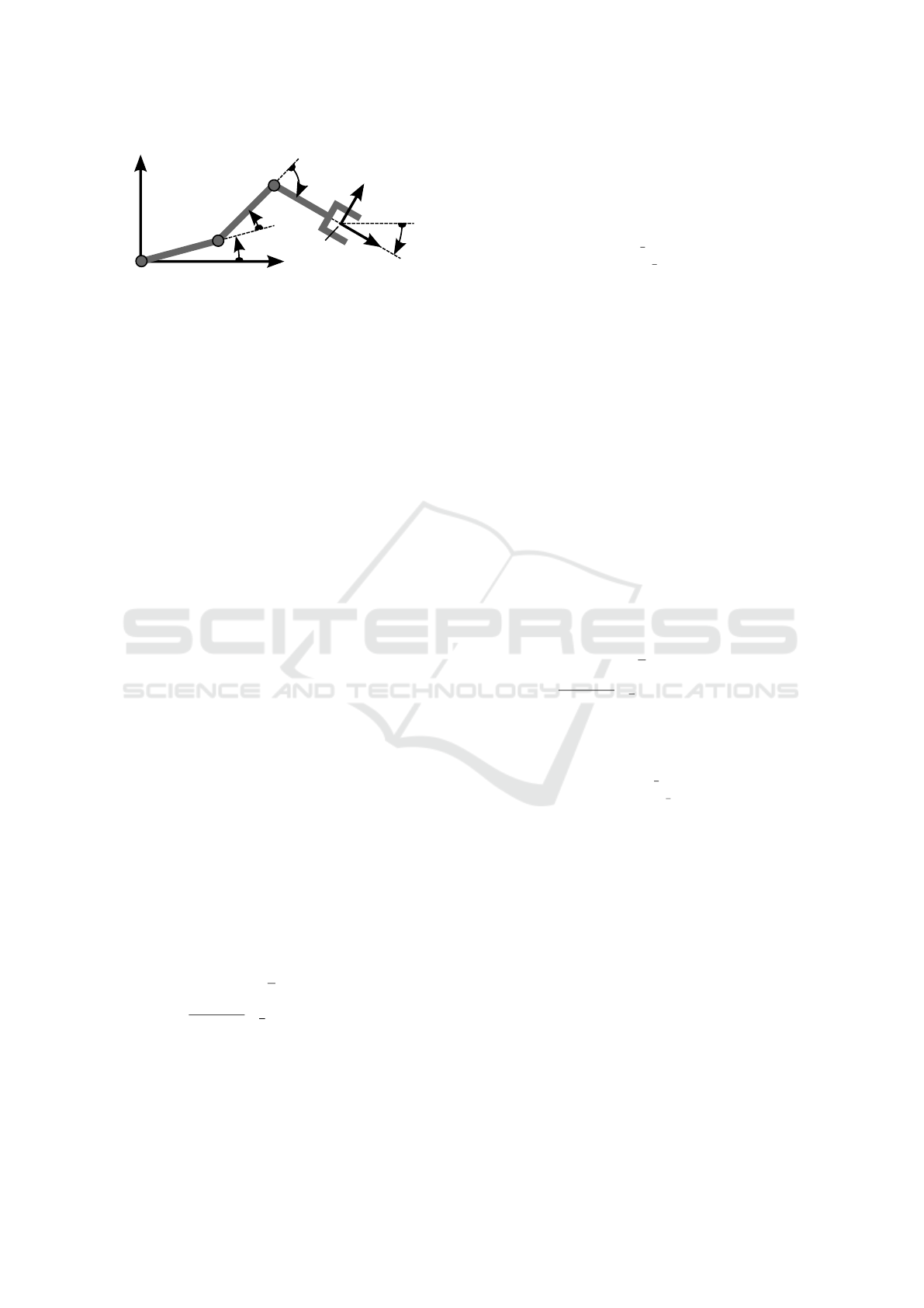
To illustrate the concepts introduced in section 3, a

planar 3-DoF manipulator is considered; see Figure

1. For the end-effector (EE), position (x, y) and ori-

entation α are considered as workspace coordinates

η = (x, y,α)

and three joint angles as joint variables

q = (θ

,θ

)

. To simplify the kinematics, we as-

sume l

= l

= 1.

The direct kinematics calculate to

f : q 7→η

η =



123

+θ



ICINCO 2023 - 20th International Conference on Informatics in Control, Automation and Robotics

332

−θ

−α

Figure 1: Planar 3-DoF Ellbow-Manipulator.

with the usual abbreviations: c

= cos θ

, c

cos(θ

+ θ

),···. Then the Jacobian follows to

J(q) =

−s

123

−s

123

−s

123

1 1 1

with singularities for θ

∈ {0,±π}. The IK solutions

on these singular conﬁgurations might not be unique.

For instance, when θ

= 0, we have a unique IK solu-

tion for a ﬁxed η

η:

(η

η) = arctan2 (x −c

,y −s

(η

η) = 0,

(η

η) = α −θ

(η

η).

On the contrary, when θ

= π, we have an inﬁnite

number of solutions represented by the straight line:

+ θ

= α − π. For the latter case, the singu-

larity locus becomes a helix in the workspace S =

{(x,y,α)|x = c

∧y = s

∧α = R}, with s

= sin(α)

and c

= cos(α). Hence, on θ

= 0, we have a unique

IK solution but rank loss, while on θ

= π, we have

rank loss and an inﬁnite number of solutions of IK.

5.1 System Representation

5.1.1 Case θ

= π

With θ

+θ

= α−π the Jacobian becomes

∗

(θ

, α) =

−s

−c

1 1 1

with Null space

∗

(θ

, α)



−1 0 1



= 0 and nor-

mal vector to the plane of admissible motions

∗T

(θ

, α)



−c

−s



= 0 . (20)

A normalized orthogonal matrix is given by

∗

(θ

,θ

) =



−c

−bc

−s

0 1 s



with b =

√

3−cos(2θ

)

√

2. Its ﬁrst two columns span

R (

∗

) and the last column spans N (

∗T

) as stated in

Proposition 3.2. Inserting in the velocity kinematics

yields

∗

z =

∗

q ⇔

z =

∗T

∗

q =

1+c

b b b

0 0 0

q. (21)

Instead of the real control variables

q we intro-

duce virtual control variables ζ

ζ such that

q =

∗

ζ =





ζ with k

= (−1 0 1)

, null space of

∗

at θ

= π. If one arbitrarily chooses k

= k

= 0,

then

∗

−1

+1) −1

0 0 1

. (22)

Inserting this in (21) we obtain

z =

∗T

∗

q =

∗T

∗

ζ = diag{1, 1,0}ζ

ζ. (23)

Hence, with the matrix

∗

in (22), the decoupled

state-space representation for (5) on singularity θ

π is as follows:



˙z

˙q



= ζ

, i ∈{1, 2, 3}. (24)

5.1.2 Case θ

= 0

With θ

+ θ

= α and θ

= 0, the Jacobian becomes

∗

(θ

, α) =



−2s

−s

1 1 1



The null space of the Jacobian and a vector that is nor-

mal to the plane of admissible motions are (1 −2 1)

and (c

)

respectively. Similar to the previous

case, a normalized orthogonal matrix

∗

can be set

up using the normal vector of the plane of motion by

∗

(θ

, θ

) =



−bc

0 −1 s



with b =

√

3−cos(2θ

)

√

2, whose ﬁrst two columns

span R (

∗

) and the last column spans N (

∗T

). Fol-

lowing all steps stated in proposition 3.2, we end up

again with (24) and the virtual control law

q =

∗

ζ =

−1

+1) 1

−2

0 0 1

ζ.

5.2 Controllability

Next, for this example, the function in (19)

is deﬁned as Φ(q) = det(

J) = s

. The pres-

ence of a time-invariant subset implies that

Φ =

∂Φ(q)

/∂q

q =



0 c



∗

ζ = 0. To stay on sin-

gular space, we set ζ

= ζ

= 0 and it follows



0 1 0





= 0. This requires k

0 and according to Lemma 4.2, internal motion exists,

otherwise not.

For the case θ

= π, it is evident that k

= 0 and

it also implies

= 0. Thus, a ﬁnitely extended jour-

ney in null space is possible, and identiﬁed as Type-1

singularity. On the other hand, for θ

= 0 we have

nonzero k

. Hence, in this case, self-motion doesn’t

exist and is identiﬁed as Type-2 singularity.

Preliminary Results on Controllability of Serial Robot-Manipulators in Singular Conﬁgurations

333

Next, we investigate what type of controllability

we have on Type-1 and Type-2 singularities for this

example. Before moving forward, it is still unclear

whether internal motion on Type-1 singularity per-

mits coverage of the entire admissible direction in the

workspace. For a pure null space motion, we have

= ζ

= 0. Then, the corresponding motion in joint

space is

= −ζ

= 0,

= ζ

. This is in-

tegrable over time so that θ

= −ζ

t −ζ

, θ

= ζ

t + ζ

. Inserting into normal vector

(20) yields

n(t) =



−cos (−ζ

t−ζ

)

−sin (−ζ

t−ζ

)

sin(ζ

t+ζ

)





−cos(φ)

sin(φ)



It sufﬁces to ﬁnd at least two values for φ

so that the corresponding n are linearly inde-

pendent. This is given by φ ∈ {0, π}: n ∈

{



−1 0 0





0 1 1



}. Since the two variants

of n are linearly independent, this holds also for the

corresponding vectors n ×j

. This proves that along

a null space motion, we can go in any direction.

We now have the necessary tools to specify con-

trollability on singularities. On a Type-2 singularity,

we can only move in the null space motion direction.

As a result, we can pass the singularity, but cannot

follow all the desired trajectories. In this situation,

we have only local accessibility. On Type-1 singular-

ities, on the other hand, we can move in any direction

by changing the null space motion direction, and we

can follow any desired trajectories. As a result, in

this instance, we have local controllability. However,

we cannot instantly follow trajectories since modify-

ing the conﬁguration with the internal motion takes

some time to obtain the desired null space motion di-

rection. As a result, on Type-2 singularities, we have

local controllability but not small-time local control-

lability(STLC).

6 SUMMARY AND OUTLOOK

This work considers control issues in robot motion

planning instead of avoiding singular conﬁguration

when the desired trajectory passes through singular-

ities. We proposed a method for totally decoupling

velocity kinematics representation for planner robot-

manipulators on singularities. The proposed method

is particularly attractive for analytical computation

since it doesn’t need SVD. An interesting outcome is

the classiﬁcation of singularities based on their con-

trollability property. The limitation of this result is we

can only classify singularities for the example we are

considering here. Yet, the observations could lead to

some interesting possibilities. We are conﬁdent that

achieving local controllability is possible in various

kinds of internal singularities. This line of research

will be expanded in the future.

REFERENCES

Chang, K.-S. and Khatib, O. (1995). Manipulator control

at kinematic singularities: A dynamically consistent

strategy. IEEE/RSJ International Conference on Intel-

ligent Robots and Systems. Human Robot Interaction

and Cooperative Robots, pages 84–88.

Conkur, E. and Buckingham, R. (1997). Clarifying the def-

inition of redundancy as used in robotics. Robotica,

15:583 – 586.

Huang, Y., Yong, Y. S., Chiba, R., Arai, T., Ueyama, T.,

and Ota, J. (2016). Kinematic control with singular-

ity avoidance for teaching-playback robot manipula-

tor system. IEEE Transactions on Automation Science

and Engineering, 13:729–742.

Kieffer, J. (1994). Differential analysis of bifurcations

and isolated singularities for robots and mechanisms.

IEEE Transactions on Robotics and Automation,

10:1–10.

Kuo, C. J., Ting, K.-C., and Chen, Y.-C. (2017). State of

product detection method applicable to industry 4.0

manufacturing models with small quantities and great

variety: An example with springs. International Con-

ference on Applied System Innovation (ICASI), pages

1650–1653.

Mareczek, J. (2020). Local optimal tracking control for ma-

nipulators with restrictive joint velocity and accelera-

tion limits. IEEE/ASME International Conference on

Advanced Intelligent Mechatronics (AIM), pages 230–

237.

Mazzanti, M., Cristalli, C., Gagliardini, L., Carbonari, L.,

Lattanzi, L., and Massa, D. (2019). A novel trajec-

tory generation algorithm for robot manipulators with

online adaptation and singularity management. IEEE

28th International Symposium on Industrial Electron-

ics (ISIE), pages 1115–1120.

Nahavandi, S. (2019). Industry 5.0 - a human-centric solu-

tion. Sustainability, 11.

Nielsen, L., de Wit, C. C., and Hagender, P. (1991). Con-

trollability issues of robots in singular conﬁgurations.

IEEE International Conference on Robotics and Au-

tomation, pages 2210–2215.

Oetomo, D. and Ang, M. H. (2009). Singularity robust algo-

rithm in serial manipulators. Robotics and Computer-

Integrated Manufacturing, 25:122–134.

Raineri, C. G. and Bianco, M. L. (2017). An automatic sys-

tem for the avoidance of wrist singularities in anthro-

pomorphic manipulators. 13th IEEE Conference on

Automation Science and Engineering (CASE), pages

1302–1309.

Spong, M. W., Hutchinson, S., and Vidyasager, M. (2020).

Robot Modeling and Control. John Wiley & Sons,

Ltd., secoind edition.

Wampler, C. (1986). Manipulator inverse kinematic solu-

tions based on vector formulations and damped least-

squares methods. IEEE Transactions on Systems,

Man, and Cybernetics, 16:93–101.

ICINCO 2023 - 20th International Conference on Informatics in Control, Automation and Robotics

334