Hand-Drawn Diagram Correction Using Machine Learning

Tenga Yoshida

1 a

and Hiroyuki Kobayashi

2 b

Graduate School of Robotics and Design, Osaka Institute of Technology, Osaka, Japan

Department of System Design, Osaka Institute of Technology, Osaka, Japan

Keywords:

Machine Learning, Hand-Drawn Diagram, Time Series Data.

Abstract:

This paper introduces a real-time correction technique for hand-drawn diagrams on tablets, leveraging machine

learning to mitigate inaccuracies caused by hand tremors. A novel fusion of classiﬁcation and regression mod-

els is proposed; initially, the classiﬁcation model discerns the geometric shape being drawn, aiding the regres-

sion model in making precise corrective predictions during the drawing process. Additionally, a unique Mean

Angle of Vector (MAV) loss function is introduced to minimize angle changes in vectors formed by consec-

utive points, thereby reducing hand tremors especially in straight line segments. The MAV function not only

facilitates real-time corrections but also preserves the drawing ﬂuidity, enhancing user satisfaction. Experi-

mental results highlight improved correction accuracy, particularly when employing classiﬁcation alongside

regression. However, the MAV function may round off sharp corners, indicating areas for further reﬁnement.

This work paves the way for more intuitive and user-friendly digital sketching and diagramming applications.

1 INTRODUCTION

Hand-drawn diagrams on tablet devices are recog-

nized as intuitive and convenient. However, a greater

susceptibility to shakes is observed compared to tradi-

tional paper-based drawing. As a result, various hand-

shake correction methods have been developed. One

notable method that has been employed is the mov-

ing average process. In this method, the output point

is computed from the moving average of the preced-

ing and subsequent n steps for the input point at time

t. Advanced methods, wherein the ﬁlter size n is ad-

justed based on the path’s curvature, have also been

introduced (Kawase et al., 2012). Predictions can be

made using past coordinate data by these methods, but

the prediction of speciﬁc shapes remains a challenge.

Moreover, in applications designed for the correc-

tion of hand-drawn ﬁgures, the shape is typically clas-

siﬁed after being drawn, and corrections are then ap-

plied. This approach ensures that geometric ﬁgures

are drawn without imperfections such as shakes or

blurs. However, pauses in prediction are often intro-

duced, leading to a less ﬂuid drawing experience.

In the realm of hand-drawn diagram correction,

most existing methods have been centered around

bitmap images. The novelty of this research lies in

https://orcid.org/0009-0002-2766-1493

https://orcid.org/0000-0002-4110-3570

leveraging vector data for real-time correction, a facet

that has not been extensively explored before. This

vector-based approach is anticipated to offer better

accuracy and efﬁciency in correcting hand-drawn di-

agrams on digital mediums.

In response to the challenges aforementioned, it

was recognized that online hand-drawn ﬁgures can be

treated as time series data. A proposal has been made

to utilize machine learning for real-time regressive

path predictions, allowing corrections to be made dur-

ing the drawing process. This research further aims to

enhance correction accuracy by introducing concur-

rent classiﬁcation prediction. This allows the regres-

sion prediction model to adapt based on the type of

ﬁgure drawn.

2 RELATED WORK

Up to now, numerous applications of machine learn-

ing to hand-drawn data, often utilizing datasets like

MNIST, have been reported. Distinct from these stud-

ies that rely on bitmap images, the present research

is characterized by its emphasis on vector images for

correction.

When attention is given to the correction of hand-

drawn ﬁgures and time series prediction, several per-

tinent studies can be identiﬁed.

346

Yoshida, T. and Kobayashi, H.

Hand-Drawn Diagram Correction Using Machine Learning.

DOI: 10.5220/0012239300003543

In Proceedings of the 20th International Conference on Informatics in Control, Automation and Robotics (ICINCO 2023) - Volume 1, pages 346-351

ISBN: 978-989-758-670-5; ISSN: 2184-2809

2.1 Sketch-RNN

Sketch-RNN, a model based on a recurrent neural net-

work, was developed by (Ha and Eck, 2017). This

model captures the movement of the pen as time se-

ries data and is capable of generating new sketches

accordingly. The concept behind Sketch-RNN has

been extended in the current research to address

real-time ﬁgure correction. While the Sketch-RNN

methodology employs both Long Short-Term Mem-

ory (LSTM)(Hochreiter and Schmidhuber, 1997) and

Variational Autoencoder (VAE) for time series predic-

tion, only the LSTM, deemed essential for time series

prediction, is utilized in this study.

2.2 Multivariate Time Series

Transformer

Conversely, a novel framework for multivariate

time series representation learning, based on the

transformer encoder architecture, was proposed by

(Zerveas et al., 2021) in their study titled “A

Transformer-based Framework for Multivariate Time

Series Representation Learning”. This framework in-

corporates an unsupervised pre-training scheme and

has been shown to offer signiﬁcant performance ad-

vantages for supervised learning by leveraging exist-

ing data samples. In the present research, time se-

ries data of two variables, x and y coordinates, is

employed, aligning perfectly with the aforementioned

framework and task. Although it has not been adopted

in this iteration, the framework holds potential value

for the current study.

3 THEORY

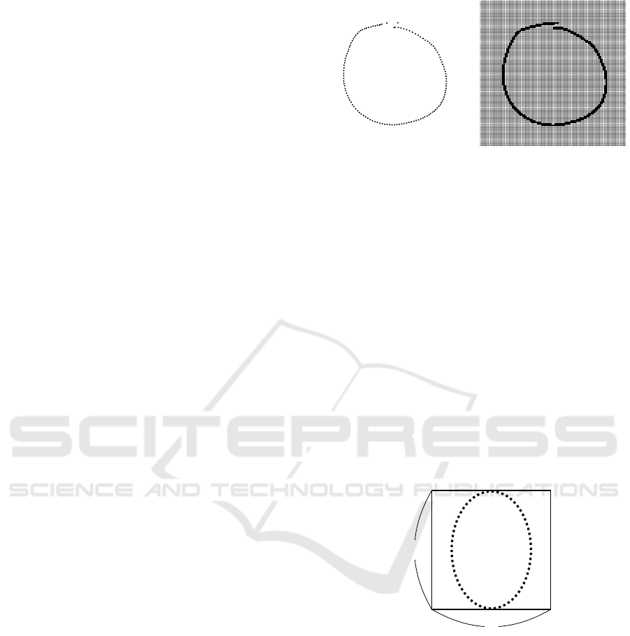
3.1 Online Patterns and Ofﬂine Patterns

Hand-drawn ﬁgure patterns can be categorized into

online patterns and ofﬂine patterns (Zhu and Naka-

gawa, 2012). Online patterns, as depicted in Fig-

ure 1a, are comprised of time series pen point co-

ordinate data, referred to here as paths. Conversely,

ofﬂine patterns, shown in Figure 1b, are made up of

pixel value data from a single image. In this study,

we utilize data from hand-drawn ﬁgures consisting of

online patterns.

3.2 Normalization

Variability in size due to feature values may cause

larger features to disproportionately inﬂuence the re-

sult, independent of their weights. The ﬁgures in

(a) Online Pattern. (b) Ofﬂine Pattern.

Figure 1: Examples of online and ofﬂine patterns.

this study also demonstrate size variations, with each

time’s coordinates (or vectors) used as the feature

values. Consequently, merely shifting the same ﬁg-

ure (changing its position) might impact the compu-

tational outcome.

For ofﬂine patterns, normalization can be

achieved by dividing each pixel value by its maxi-

mum. However, this approach does not suit the on-

line patterns utilized here. It neither addresses the is-

sue of different ﬁgure positions nor prevents changes

in the aspect ratio. Therefore, we employ normaliza-

tion using a bounding box. This box, illustrated in

Figure 2, represents the smallest square enclosing the

ﬁgure. Paths are shifted so that the ﬁgure box’s top-

left corner aligns with the origin, and all points are

normalized to lie between 0 and 1 by dividing by the

box’s length l.

Figure 2: A Example of Bounding Box.

3.3 Correction Method

Correction of hand-drawn paths involves predicting

these paths using a machine learning model. This

model comprises two components: a classiﬁcation

model and a regression model. The correction pro-

cess unfolds as follows:

1. The classiﬁcation model predicts what type of ﬁg-

ure the online pattern of the hand-drawn ﬁgure is.

2. The path of the hand-drawn ﬁgure is passed to the

regression prediction model suitable for the type

predicted by the classiﬁcation model.

Hand-Drawn Diagram Correction Using Machine Learning

347

3. The regression prediction model predicts the cor-

rected path from the path of the hand-drawn ﬁg-

ure.

4. Repeat steps 1 to 3.

The models’ input and output images are portrayed in

Figure 3.

Input

Classication

Model

For Triangle

For Line

For Ellipse

︙

Output

Regression Model

Figure 3: Classiﬁcation and regression model.

To enable real-time predictions during writing, the

machine learning model must receive inputs of con-

sistent array lengths. This necessitates data shap-

ing into x, y coordinates with an array length of 512,

meaning the model accepts inputs in the format 512×

2. Linear interpolation is employed during the data

shaping phase. Training utilizes data from ﬁve ﬁg-

ure types: straight line, triangle, square, circle, and

ellipse.

3.4 Loss Function

In previous studies (Yoshida and Kobayashi, 2022),

the Mean Square Error (MSE) was used as the loss

function given by

MSE =

length

∑

i=1

length

∑

t=0



prediction

t+i

− p

teacher

t+i



(1)

This is to bring the handwritten path closer to the

teacher path at each time. In contrast, this study intro-

duces a new loss function. Until now, there has been

no quantitative evaluation indicator for the standing.

Therefore, it was decided to incorporate the change

in the angle of the vector at each time into the loss

function. This loss is named Mean Angle of Vector

(MAV) in this study, and is represented by

MAV = γ ·

∑

i=1

cos

−1

(COS) (2)

COS =

length − 2 × n steps

length−n steps

∑

t=n steps

t+n steps

− p

) · (p

− p

t−n steps

)



t+n steps

− p



− p

t−n steps



(3)

MAV takes the difference of the vectors of the points

before and after n steps, and calculates their angles

based on the inner product. In other words, it is equiv-

alent to ﬁnding θ as shown in Figure 4. By applying

MAV only to prediction, it minimizes the change in

the angle at each point and suppresses hand shaking.

γ is the weight of MAV, and it was set to 0.001 in the

loss during training. MAV is an indicator of shaking,

and MAV is also used as metrics, but in that case, γ is

set to 1. Also, n steps was set to 5.

t−n steps

t+n steps

− p

t−n steps

t+n steps

− p

Figure 4: The angle of the vector at each time.

The ﬁnal loss is the sum of MAV and MSE, repre-

sented by Eq. (4).

Loss = MSE + MAV (4)

4 EXPERIMENT

4.1 Classiﬁcation Model

First, we conducted experiments with the classiﬁca-

tion model alone. We predicted the type of data after

10% of the path array length (for data of length 100,

this is from time 10 onwards). The accuracy of this

model was about 33%.

Predictions were then made for data after 50% of

the path array length, and the accuracy achieved was

about 60%.

Predictions made after 80% of the path array

length yielded an accuracy of about 76%.

Additionally, we made predictions using only the

ﬁnal path, which refers to the completed ﬁgure. The

accuracy for this approach was about 97.2%. The de-

tailed breakdown can be seen in Table 1. It’s evident

that the accuracy of the classiﬁcation model increases

as it approaches the end of the drawing.

Table 1: Classiﬁcation results.

OUT

line

tri-

angle

rect-

angle

circle ellipse

line 929 0 1 0 0

triangle 0 972 2 0 2

rectangle 0 1 918 0 4

circle 0 0 2 909 25

ellipse 0 0 3 121 787

ICINCO 2023 - 20th International Conference on Informatics in Control, Automation and Robotics

348

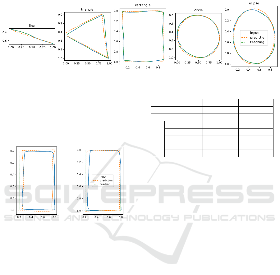
Figure 5: Results of combining classiﬁcation and regression models.

4.2 Combined Use of Classiﬁcation and

Regression Models

The results from combining the classiﬁcation and re-

gression models are presented in Figure 5.

Comparisons of results with and without classiﬁ-

cation can be viewed in Figure 6.

(a) Without classiﬁcation. (b) With classiﬁcation.

Figure 6: Comparison of results with and without classiﬁ-

cation.

4.3 Loss Using MAV

The results using the loss with MAV are depicted in

Figure 7. These were obtained exclusively with the

regression model, without the inclusion of the classi-

ﬁcation model.

The following ﬁgure, Figure 8, compares the cor-

rection results obtained using MAV and those using

MSE only.

A zoomed-in version focusing on the straight line

from Figure 8(i) is presented in Figure 9.

Similarly, a zoomed-in version focusing on the

corner from Figure 8(ii) is presented in Figure 10.

Lastly, Table 2 presents the MAV and MSE val-

ues when validation data is fed into each respective

model. The “Base Model” here represents a model

without classiﬁcation prediction and without training

using MAV.

Table 2: Classiﬁcation results.

Model type MSE MAV [rad]

Base Model 1.2310e-04 0.2852

Model with MAV 9.5786e-05 0.1490

With classify

line 1.6718e-04 0.6486

triangle 3.2093e-04 0.2167

rectangle 1.0126e-04 0.2381

circle 4.0689e-04 0.1630

ellipse 2.9909e-04 0.3540

5 DISCUSSION

Also, in the task of classiﬁcation only, the accuracy

increased as it approached the end of the drawing.

This is thought to be because the ﬁgure is accurately

formed as the drawing progresses, which enabled ac-

curate classiﬁcation. However, in the prediction while

drawing, it is necessary to increase the accuracy from

the beginning of the drawing, and this low accuracy

at the beginning of the drawing will become a bottle-

neck.

Looking at Figure 6, it can be seen that a closer

correction result to the teacher path is obtained when

classiﬁcation is performed than when it is not per-

formed. This conﬁrmed that the correction accuracy

improved by performing classiﬁcation. However, for

each regression prediction model, there is a tendency

for overﬁtting, and it is believed that generality has

been lost.

Next, looking at the results using the loss function

with MAV, it is not signiﬁcantly improved as seen in

Figure 8. However, looking at Figures 9 and 10, it

can be seen that the hand tremor is reduced in each.

However, looking at Figure 10, it can be seen that the

corners are rounded when using MAV. This is thought

to be because the corners are rounded by suppressing

the change in angle at each time. In other words, this

method is thought to have a similar effect to the mov-

ing average method.

Hand-Drawn Diagram Correction Using Machine Learning

349

Figure 7: Results using loss with MAV.

(a) MSE only. (b) With MAV.

Figure 8: Comparison of results using MAV and MSE only.

(a) MSE only. (b) With MAV.

Figure 9: Comparison of results using MAV and MSE only

(zoomed in on the straight line, only prediction).

(a) MSE only. (b) With MAV.

Figure 10: Comparison of results using MAV and MSE only

(zoomed in on the corner, only prediction).

For shapes other than straight lines, it is not al-

ways good for MAV to be 0, so this method is thought

to have room for improvement. For example, de-

signing a loss function to bring the distribution of

MAV closer to a normal distribution using the Kull-

back–Leibler divergence may result in better results.

Looking at Table 2, it can be seen that when the

loss function using MAV is used, the value of MAV

decreases signiﬁcantly. This result is consistent with

the result in Figure 8. However, in the case of the

model using classiﬁcation, the value of MAV ﬂuctu-

ates greatly. These need to be veriﬁed in the future.

6 CONCLUSION

In this study, we introduced a method that combines

classiﬁcation prediction with traditional regression

prediction. While we observed an improvement in

accuracy over the conventional approach, the classi-

ﬁcation model’s accuracy remained suboptimal. Fur-

thermore, the large model size resulted in longer cor-

rection times, posing potential challenges for applica-

tions on mobile devices. Addressing these issues is an

area of ongoing consideration.

We also proposed a loss function using MAV.

While MAV proved effective in reducing hand

tremors for straight-line segments, it introduced is-

sues like rounding at the corners. Nevertheless, as

MAV has not undergone quantitative evaluation to

date, we still regard it as a promising metric for as-

sessing hand tremors.

Looking ahead, we are exploring the adoption

of the Transformer architecture, which has gained

prominence in recent natural language processing en-

deavors, to enhance our classiﬁcation model’s accu-

racy and reduce its size. The recursive models, such

as LSTM and RNN, employed in this study are adept

at handling time series data. However, they suffer

from information loss as input sequences grow. In

contrast, the Transformer’s performance is not dic-

tated by input length, allowing it to maintain data

ﬁdelity over extensive sequences. This trait sug-

ICINCO 2023 - 20th International Conference on Informatics in Control, Automation and Robotics

350

gests that employing Transformers can optimize pre-

dictions with fewer parameters, leading to a more

streamlined model. Future work will focus on lever-

aging the Transformer, as discussed in (Zerveas et al.,

2021), to elevate our classiﬁcation model’s accuracy

and decrease its overall footprint.

REFERENCES

Ha, D. and Eck, D. (2017). A neural representation of

sketch drawings. arXiv preprint arXiv:1704.03477.

Hochreiter, S. and Schmidhuber, J. (1997). Long short-term

memory. In Neural Computation. MIT Press.

Kawase, H., Shinya, M., and Shiraishi, M. (2012). Beau-

tiﬁcation of hand-drawn strokes by adaptive moving

average for illustration trancing tasks. In The Institute

of Image Information and Television Engineers Tech-

nical Report. The Institute of Image Information and

Television Engineers.

Yoshida, T. and Kobayashi, H. (2022). Correction of online

handwriting stroke using machine learning. In The

Proceedings of JSME annual Conference on Robotics

and Mechatronics (Robomec). The Japan Society of

Mechanical Engineers.

Zerveas, G., Jayaraman, S., Patel, D., Bhamidipaty, A., and

Eickhoff, C. (2021). A transformer-based framework

for multivariate time series representation learning. In

Proceedings of the 27th ACM SIGKDD conference on

knowledge discovery & data mining. Association for

Computing Machinery.

Zhu, B. and Nakagawa, M. (2012). Recent trends in online

handwritten character recognition. In The Journal of

the Institute of Electronics, Information and Commu-

nication Engineers. The Institute of Electronics, Infor-

mation and Communication Engineers.

Hand-Drawn Diagram Correction Using Machine Learning

351