Study on Cost Estimation of the External Fleet Full Truckload Contracts

Jan Kaniuka

1 a

, Jakub Ostrysz

1 b

, Maciej Groszyk

1 c

, Krzysztof Bieniek

1 d

Szymon Cyperski

2 e

and Paweł D. Doma

nski

1,2 f

Warsaw University of Technology, Institute of Control and Computation Engineering,

Nowowiejska 15/19, 00-665 Warsaw, Poland

Control System Software Sp. z o.o., ul. Rzemie

slnicza 7, 81-855 Sopot, Poland

Keywords:

Cost Estimation, Full Truck Loads, Machine Learning, Regression, kNN, Decision Trees, Gaussian Processes.

Abstract:

Goods shipping supports the operation and the development of the global economy. As there are thousands

of logistics companies, there exists a big need for solutions for their daily operation. The shipment can be

carried out in many ways. This work focuses on the road transportation in form of the Full Truck Load (FTL).

Once the service is supported by the third party, there is a need to have a tool that compares various offers

and allows to estimate the cost. Generally, FTLs are used in the long range routes and the estimation of such

contracts can be handled in many ways starting from the simple calculators up to data based machine learning

solutions. Nonetheless, the need for the cost estimation appears for the short routes, which often support long

range ones. Their pricing rules differs from the long range ones and the required approaches should differ as

well. This work presents the wide comparison of 35 regression and machine learning approaches applied to

the task. The assessment is performed using real contract data of several companies operating in Europe.

1 INTRODUCTION

Full truckload (FTL) is a common transportation way,

where the goods ﬁll an entire truck. It ideally suits for

large volume of goods where a load covers the whole

truck space. There is an alternative approach called

less than truckload (LTL), in which a truck takes par-

tial loads to different contract load/unload locations

within a single travel. This paper focuses on the FTL

approach, however from a rare perspective.

First of all, the case of external ﬂeet contract pric-

ing is considered. It is assumed the contractor may

use some custom dynamic pricing model, which is

associated with serious challenges (Stasi

nski, 2020).

These issues become even more signiﬁcant in the case

of short routes, when common relationships with the

fuel costs and driver time start to matter much less.

External ﬂeet long range contracts pricing can be

solved with the use of popular fright cost calculators

https://orcid.org/0009-0009-9379-4906

https://orcid.org/0009-0006-8178-0134

https://orcid.org/0009-0006-4050-6585

https://orcid.org/0009-0007-5232-3628

https://orcid.org/0009-0009-5655-7143

https://orcid.org/0000-0003-4053-3330

or using the artiﬁcial intelligence (AI) and machine

learning (ML) (Tsolaki et al., 2022).

The task of the short range external ﬂeet FTL ship-

ment cost estimation, is not speciﬁcally addressed in

the literature. Actually, this subject is hidden behind

the general FTL estimation and people practically do

not distinguish short routes cost prediction as sepa-

rate task. The ﬁndings that appeared during the in-

vestigation of this project repeat despite the method

used. The biggest challenge in the FTL cost predic-

tion is that the highest estimation residua appear for

the short routes and low costs. The shorter the route,

the more difﬁcult it is to be estimated. The general

absolute performance measures are low, while the rel-

ative ones appear to be suspiciously high. This hap-

pens due to the possible high share of the low cost

routes. Thus, we have decided to take a closer look at

this subject decomposing the problem into two sub-

problems. This work copes with the problem of the

short routes, while the longer ones are already cov-

ered in (Cyperski et al., 2023). Concluding, our work

aims to ﬁll this gap. General FTL cost estimation ap-

proaches are introduced in Section 2. The case study

and used data are presented in Section 3. This work

compares 35 various estimators described in Section

316

Kaniuka, J., Ostrysz, J., Groszyk, M., Bieniek, K., Cyperski, S. and Doma

nski, P.

Study on Cost Estimation of the External Fleet Full Truckload Contracts.

DOI: 10.5220/0012251000003543

In Proceedings of the 20th International Conference on Informatics in Control, Automation and Robotics (ICINCO 2023) - Volume 2, pages 316-323

ISBN: 978-989-758-670-5; ISSN: 2184-2809

4, which are applied to the task. Section 5 analyzes

the results, while the work is concluded in Section 6.

2 DYNAMIC FTL PRICING

The FTL freight cost estimation model is needed

as external ﬂeets use dynamic pricing strategies

(Stasi

nski, 2020). Any information about cost inﬂu-

ential factors helps, especially in its structure evalu-

ation and features selection. One should consider a

combination of general and custom market and non-

market factors (Vu et al., 2022). Proper selection of

the inﬂuencing features improves the estimation.

Contract dependent factors are included in the

order limiting the solution. They may address the

type of the truck and required speciﬁc equipment,

ADR (l’Accord europ

een relatif au transport inter-

national des marchandises Dangereuses par Route –

transport with hazardous materials) or drivers’ certiﬁ-

cates. Shipping load and unload locations determine

the route. The location and the contract timeframe

has to be matched with the drivers availability. The

contract also deﬁnes the payment terms. The litera-

ture focuses on the blind machine learning approaches

(Pioro

nski and G

orecki, 2022; Tsolaki et al., 2022) or

more complex hybrid ones (Cyperski et al., 2023).

3 ESTIMATION CASE STUDY

The data used to evaluate and test the method orig-

inated from the databases for selected Polish trans-

portation companies (Janusz et al., 2022). Original or-

ders database consists of approximately 414,000 po-

sitions. The data considered are limited only to the

short range contracts, which limits the number of data

to 20,239 records from the time period from January

, 2016 to April 30

, 2022. These record are con-

sidered as the training data. Records from May 1

2022 till August 1

, 2022 are considered as the val-

idating dataset. Therefore, we obtain 703 records in

the validating dataset (see Table 1).

Table 1: Size of datasets used in experiments.

Raw data Preprocessed data

Train set 414 404 20 239

Test set 14 968 703

3.1 Data Preprocessing

Each registered contract is described by 22 variables

from the production databases. While modeling the

transportation cost, we limit this number to 12 the

most important features: date of payment, min and

max transport time, time interval, date of transport,

lead time, total and total empty distances, number of

pickups and unloadings, demand for cold storage and

fuel-cost. The following descriptors are excluded:

• ID number → it is just a sequence number,

• maximum weight and tonne-kilometres → these

data are frequently incomplete, and cannot be

practically used,

• location cluster number (Cyperski et al., 2023),

the latitudes and longitudes of the loading and un-

loading site → are used only in the selection of

the short range contracts.

Python programming language (scikit learn and

torch libraries) and MATLAB (Statistics and Machine

Learning Toolbox) are used during data processing

and the estimation process.

4 ESTIMATION APPROACHES

This section describes the machine learning ap-

proaches taken into account during the study. The

choice of black box approaches is motivated by the

unknown pattern behind the data due to the dynamic

geopolitical situation and the speciﬁcity of the very

short shipping. Among other factors, rising inﬂation,

Brexit and the COVID-19 pandemic are impacting

truck cargo transit prices. The following regression

estimation methods are taken into account:

– regression approaches:

LMS: Least Mean Squares,

R-LMS: Robust Linear Regression, which is ro-

bust against outliers

(Holland and Welsch, 2007),

SLR: Stepwise Linear Regression

(Yamashita et al., 2006),

TS-LR: Theil-Sen Regression

(Wang et al., 2009),

H-LR: Huber Regressor

(Huber and Ronchetti, 2011),

– support vector machines (Wang and Hu, 2005):

LSVM: Linear Support Vector Machines,

KSVM: Kernel Support Vector Machines,

QSVM: Quadratic Support Vector Machines,

CGSVM: Coarse Gaussian Support Vector Ma-

chines,

MGSVM: Medium Gaussian Support Vector

Machines,

Study on Cost Estimation of the External Fleet Full Truckload Contracts

317

FGSVM: Fine Gaussian Support Vector Ma-

chines,

– Gaussian processes (Schulz et al., 2018):

EGPR: Exponential Gaussian Process,

SEGPR: Squared Exponential Gaussian Process

Regression,

MGPR: Matern 5/2 Gaussian Process Regres-

sion,

RGPR: Rational Quadratic Gaussian Process

Regression,

– k-NN: k-Nearest Neighbors Regressor

(Yao and Ruzzo, 2006),

– OMP Orthogonal Matching Pursuit

(Tropp, 2004),

– ridge regressions (Li et al., 2020):

RR: Ridge Regression,

ARD-RR: Automatic Relevance Determination,

B-RR: Bayesian Ridge Regression,

– decision trees (Breiman et al., 1984):

DTR: Decision Tree Regressor

(Breiman, 2017),

BoostRT: Boosted Regression Trees

(Bergstra et al., 2012),

GBoostRT: Gradient Boosting Regression

(Friedman, 2001),

HGBoostRT: Histogram Gradient Boosting Re-

gression

(Tiwari and Kumar, 2021),

ERTR: Extremely Randomized Trees

(Geurts et al., 2006),

BRTR: Bagged Regression Trees

(Sutton, 2005),

F-DTR: Fine Regression Tree,

M-DTR: Medium Regression Tree,

C-DTR: Coarse Regression Tree,

RFR: Random Forest Regression

(Ho, 1995),

– regularization techniques (Tibshirani, 1996):

LASSO-R: LASSO Regression,

LARS-R: LARS Lasso

(Efron et al., 2004),

ENR: Elastic Net Regression

(Zou and Hastie, 2005),

LAR: Least Angle Regression,

– ANN: Artiﬁcial Neural Network optimized ac-

cording to the following hyperparameters:

– number of hidden neurons: 12-2048,

– number of hidden layers: 1-8,

– activation fun.: RELu, Tanh, identity, logistic,

– optimizer: Adaptive Moment Estimation,

Stochastic Gradient Descent.

5 RESULTS

The comparison of the methods uses the residuum

analysis. Three performance measures are used:

Mean Absolute Error (MAE), Mean Absolute Per-

centage Error (MAPE) and Mean Square Error

(MSE). MAE error is deﬁned as (1), while the MSE as

(2), where y is the actual and ˆy is the predicted value.

MAE =

∑

y − ˆy

(1)

MSE =

∑

(y − ˆy)

(2)

MAPE deﬁnes the accuracy of a forecasting

method that is given by the formula (3)

MAPE =

100%

∑



y − ˆy



. (3)

Colin David Lewis proposed in (Lewis, 1982) the ta-

ble (see Table 2) containing interpretation of typical

MAPE values. MAPE as a relative error allows us to

more naturally interpret of how accurate the model is.

Table 2: Interpretations of MAPE values.

MAPE [%] Interpretation

<10 Highly accurate forecasting

10–20 Good forecasting

20–50 Reasonable forecasting

>50 Inaccurate forecasting

5.1 Comparison of the Performance

At ﬁrst, the models are simply compared by their per-

formance measures. Table 3 shows the respective val-

ues. Even the draft review brings interesting obser-

vations. First of all, each measure indicates different

models. The MSE highly penalizes residua with large

values in opposition to the small ones. It is shown (Se-

borg et al., 2010) that the MSE punishes large devia-

tions and is sensitive to the outlying observations. The

MAE is less conservative. It has the closest relation-

ship to economic considerations (Shinskey, 2002).

The difference between MAE and MAPE also re-

quires for some discussion. The fact that both indexes

indicate different regressors is due to the fact that the

errors lie in different parts of data. Minimized MAE

is due to the residua of the higher cost sacriﬁcing the

ICINCO 2023 - 20th International Conference on Informatics in Control, Automation and Robotics

318

Table 3: Comparison of the regression models. Grey color highlights the extreme values of the models: the worst (red) and

the best (green). Bold numbers indicate the worst and the best one.

No Descriptor Method Name MAE MSE MAPE [%]

1 LMS Least Squares 205.8 704903 66.24

2 R-LMS Robust Linear Regression 189.2 837335 37.69

3 SLR Stepwise Linear Regression 226.8 1664193 75.34

4 TS-LR Theil-Sen Regressor 188.4 851928 46.61

5 H-LR Huber Regressor 177.6 763898 41.4

6 LSVM Linear Support Vector Machines 175.6 764256 36.11

7 KSVM Kernel Support Vector Machines 298.9 1943548 60.79

8 QSVM Quadratic Support Vector Machines 187.1 877200 45.61

9 CGSVM Coarse Gaussian Support Vector Machines 195.6 1088107 50.5

10 MGSVM Medium Gaussian Support Vector Machines 235.0 1479565 56.79

11 FGSVM Fine Gaussian Support Vector Machines 304.8 1746572 79.59

12 EGPR Exponential Gaussian Process Regression 155.5 748644 42.58

13 SEGPR Squared Exponential Gaussian Process Regression 202.4 1193684 42.76

14 MGPR Matern 5/2 Gaussian Process Regression 182.1 967428 42.37

15 RGPR Rational Quadratic Gaussian Process Regression 159.7 718013 38.31

16 k-NN k-Nearest Neighbors Regressor 200.9 824671 57.08

17 OMP Orthogonal Matching Pursuit 198.0 858053 40.65

18 RR Ridge Regression 205.8 704902 66.24

19 ARD-RR Automatic Relevance Determination 205.4 704991 65.99

20 B-RR Bayesian Ridge Regression 205.7 704758 66.31

21 DTR Decision Tree Regressor 167.9 614842 35.45

22 BoostRT Boosted Regression Trees 164.7 719251 33.58

23 GBoostRT Gradient Boosting Regression 151.8 695577 38.04

24 HGBoostRT Histogram Gradient Boosting Regression 140.0 490936 34.01

25 ERTR Extremely Randomized Trees 131.2 712589 27.68

26 BRTR Bagged Regression Trees 128.5 626157 26.83

27 F-DTR Fine Regression Tree 161.6 688117 29.23

28 M-DTR Medium Regression Tree 140.6 675587 27.12

29 C-DTR Coarse Regression Tree 130.5 609023 26.25

30 RFR Random Forest Regression 136.1 625584 30.77

31 LASSO-R LASSO Regression 205.9 705301 66.54

32 LARS-R LARS Lasso 205.9 705301 66.54

33 ENR Elastic Net Regression 204.9 702740 66.39

34 LAR Least Angle Regression 205.8 704903 66.24

35 ANN Artiﬁcial Neural Network 134.0 651000 27.82

contracts of low cost. In contrary, minimization of the

relative error (MAPE) does not distinguish between

the contract absolute value. This observation may be

used to design estimation performance index.

Furthermore, the reference between obtained

numbers and the MAPE errors interpretation sketched

in Table 2 shows that none of models can be consid-

ered as useful for the good or highly accurate fore-

casting. The majority of them are categorized as

reasonable. Few of these reasonable models, such

as Coarse, Medium or Bagged Regression Trees are

positioned the closest to the good forecasting cate-

gory. In contrary there are some models, like the

Least Squares, Stepwise Linear Regression, the ma-

jority of Support Vector Machines, k-Nearest Neigh-

bors, ridge regression variants and regularized models

that are clearly unacceptable.

Thus, we notice that some categories of the ap-

proaches perform better, while the other ones, despite

the version applied are not able to cope with the prob-

lem. We may clearly see, that despite the applied vari-

ant decision trees deliver consistently good results,

Study on Cost Estimation of the External Fleet Full Truckload Contracts

319

in contrary to the Support Vector Machines. Linear

Regression models are characterized by high variabil-

ity in their performance. Robust Linear Regression

is twice better than the Stepwise Linear version. It

is probably due to the frequent outlying observations

in data. Artiﬁcial Neural Network model is relatively

good, however it looses against decision trees.

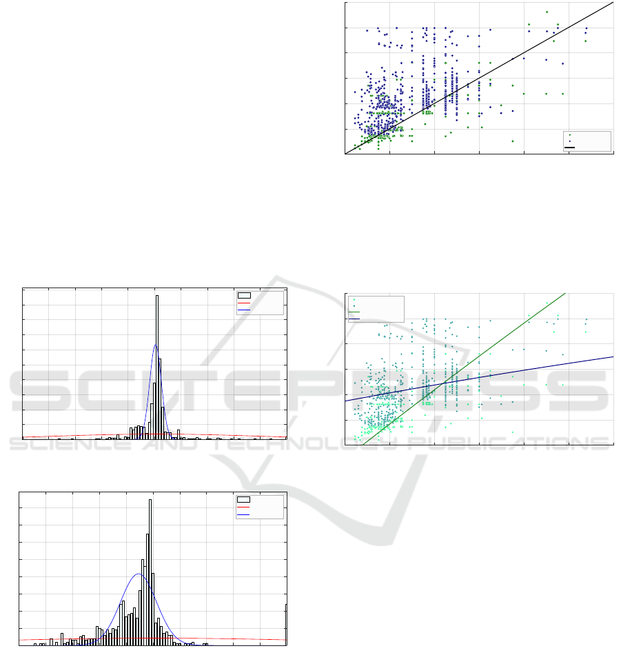
Further residuum analysis might be performed

using the comparison of the obtained residua his-

tograms. Fig.1 shows sample histograms for the

best Coarse Regression Tree and the worst perform-

ing Fine Gaussian Support Vector Machines model.

We clearly notice the non-Gaussian properties of the

residua probably due to the original process data or

the relatively small sample size. Furthermore, we ob-

serve that the results are skewed towards negative er-

rors, i.e. overestimation. We also see a lot of outlying

observations, which is reﬂected by the large differ-

ence between normal and robust version of the ﬁtted

Gaussian probabilistic density function (PDF).

-1000 -800 -600 -400 -200 0 200 400 600 800 1000

prediction error

100

120

140

160

180

200

no of occurances

histogram

normal PDF

robust PDF

(a) Coarse Regression Tree model.

-1000 -800 -600 -400 -200 0 200 400 600 800 1000

prediction error

no of occurances

histogram

normal PDF

robust PDF

(b) Fine Gaussian Support Vector Machines model.

Figure 1: Sample histogram plots for the best and the worst

models with the ﬁtted normal and robust Gaussian PDFs.

Next plot shows the predicted versus the real costs

plot analyzing the hypothesis that the error and the

quality of estimation may depend on the cost of the

shipping. Fig. 2 shows this relationship for two se-

lected models: C-DTR and FGSVM. We observe the

largest difference in the decision tree model improve-

ment is achieved for low and medium cost contracts.

0 200 400 600 800 1000 1200

real cost

200

400

600

800

1000

1200

predicted cost

C-DTR

FGSVM

ideal prediction

Figure 2: The predicted versus real cost for selected models.

It can be observed in Fig. 3, which shows the re-

lationship between prediction error and the real cost.

This dependence is well seen through the polynomial

ﬁtting the error and the real cost. To discard the effect

of outliers robust regression is used for ﬁtting.

0 200 400 600 800 1000 1200

real cost

200

400

600

800

1000

1200

estimated cost

C-DTR

FGSVM

C-DTR polynomial

FGSVM polynomial

Figure 3: The relationship between the prediction error (3

order polynomial) and the contract real cost.

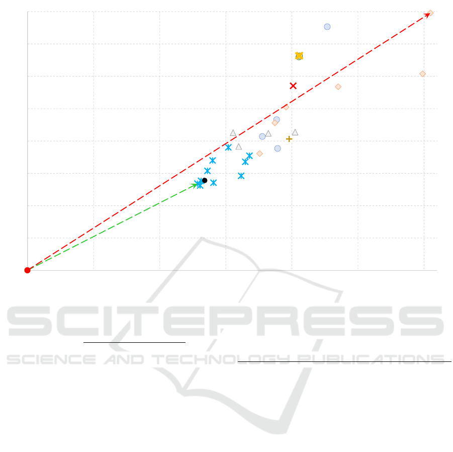
Residuum analysis is not a simple comparison be-

tween two numbers, as each measure, their relations

matter, which can be further assessed with the statisti-

cal analysis or dedicated multi-criteria plots. Clearly,

this is multi-criteria assessment. As one can see, ab-

solute and relative errors may indicate different pre-

diction models as good ones. There is a need for

an aggregating approach and the according measure.

We propose the two-dimensional plot of the relative

(MAPE) versus the absolute (MAE) measure, denoted

as Index Ratio Diagrams (IRD). The best model (pre-

dictor) is the one, which is the closest to the origin.

The distance measure is called the Aggregated Dis-

tance Measure (ADiMe). Fig. 4 presents IRD plot for

the considered FTL cost estimation models.

The general formulation of the aggregated ADiMe

index is sketched in Eq. (4). Generally, the measure

might be scaled with coefﬁcients w

and w

, which set

the ratio between the relative and the absolute index.

In the considered case both coefﬁcients are equal and

ICINCO 2023 - 20th International Conference on Informatics in Control, Automation and Robotics

320

LMS

R-LMS

SLR

TS-LR

H-LR

LSVM

KSVM

QSVM

CGSVM

MGSVM

FGSVM

EGPR

SEGPR

MGPR

RGPR

k-NN

OMP

ARD-RR

B-RR

DTR

BoostRT

GBoostRT

HGBoostRT

ERTR

BRTR

F-DTR

M-DTR

C-DTR

RFR

LASSO-RLARS-R

ENR

LAR

ANN

0 50 100 150 200 250 300

MAPE

MAE

Figure 4: The IRD plot comparing the models: red line shows the worst model (the longest distance), green the best one (the

shortest distance).

= w

= 1.

ADiMe =

· MAE

+ w

· MAPE

(4)

The colors on the plot indicates various classes of

the models. In this way, the assessment of the mod-

els is much easier, as each model is represented by a

single point in the two-dimensional plot. We clearly

see that the class of the decision tree models is the

most homogeneous and all of them achieve relatively

good performance. In contrary, the support vector

machines models represent the most scattered class,

with the biggest difference in their performance. We

also see that the ridge regression variant and the se-

lection of the regularization technique make no dif-

ference for the model property. Gaussian regression

schemes are also quite homogeneous, however their

performance is worse comparing to the decision trees.

Table 4 compares the models. It presents ordered

ﬁrst ﬁve the best models and ﬁve the worst ones as

well. We see that the difference between the methods

is signiﬁcant, as poor estimators might be three times

worse than the best one. This observation once more

conﬁrms the well-known fact that the model selection

is crucial to achieve satisfactory estimators.

Comparison of the best models is not clearly vis-

ible in the non scaled plot. Therefore, the Fig. 5

shows the same plot, but with the magniﬁed region

Table 4: Comparison of ﬁve the best and ﬁve the worst mod-

els according to the ADiMe.

rank method ADiMe MAE MAPE [%] MSE

1 BRTR 131.3 128.5 26.83 626157

2 C-DTR 133.2 130.5 26.25 609023

3 ERTR 134.1 131.2 27.68 712589

4 ANN 136.9 134.0 27.82 651000

5 RFR 139.6 136.1 30.77 625584

30 LASSO-R 216.4 205.9 66.54 705301

31 LARS-R 216.4 205.9 66.54 705301

32 SLR 239.0 226.8 75.34 1664193

33 MGSVM 241.7 235.0 56.79 1479565

34 KSVM 305.0 298.9 60.79 1943548

35 FGSVM 315.0 304.8 79.59 1746572

of the best models. It’s worth to notice that the arti-

ﬁcial neural network model (ANN) behaves similarly

to the best predictors, being ranked as the fourth best.

6 CONCLUSIONS AND FURTHER

OPPORTUNITIES

The presented work has three dimensions and conclu-

sion types. Firstly, it analyzes the issue of the short

routes external ﬂeet FTL contracts cost assessment,

which actually is hardly analysed in the literature.

Subject seems to be underrated, despite of its huge

Study on Cost Estimation of the External Fleet Full Truckload Contracts

321

R-LMS

H-LR

LSVM

EGPR

MGPR

RGPR

OMP

DTR

BoostRT

GBoostRT

HGBoostRT

ERTR

BRTR

F-DTR

M-DTR

C-DTR

RFR

ANN

120 130 140 150 160 170 180 190 200

MAPE

MAE

Figure 5: The scaled IRD plot comparing the best prediction models.

practical value. Probably it is hidden behind the gen-

eral FTL pricing, or the results are not so impressive

though being practically acceptable.

The second contribution is in fact that we were

able to ﬁnd out approaches, originating from the de-

cision trees that allow to get satisfactory models. Es-

pecially, the Coarse, Medium or Bagged Regression

Trees deliver reasonable prediction accuracy.

Finally, the obtained results are used to perform

deeper residuum analysis. It shows that an error is

not equal to the error. The speciﬁc use of the measure

may favor one method against the other and the inter-

pretation of the results can be easily biased. There-

fore, the estimation model analysis should not be lim-

ited to the simple comparison of one measure num-

bers, but further investigation using statistical meth-

ods, or just different residua presentation can help.

It is also proposed the aggregated approach to the

multi-criteria residuum analysis using the visual ap-

proach through the Index Ratio Diagrams (IRD) and

resulting Aggregated Distance Measure (ADiMe).

The analysis of the FTL shipping is still not over.

Several subjects remain open. How to improve ob-

tained models and optimize their hyperparameters?

How to improve the residuum analysis and how to get

it simpler? There is still a work to be done.

ACKNOWLEDGEMENTS

Research is supported by the Polish National

Centre for Research and Development, grant

no. POIR.01.01.01-00-2050/20, application track

6/1.1.1/2020 - 2nd round.

REFERENCES

Bergstra, J., Pinto, N., and Cox, D. (2012). Machine learn-

ing for predictive auto-tuning with boosted regression

trees. In 2012 Innovative Parallel Computing (InPar),

pages 1–9. IEEE.

Breiman, L. (2017). Classiﬁcation and Regression Trees

(1st ed.), chapter 8. Routledge.

Breiman, L., Friedman, J., Stone, C., and Olshen, R. (1984).

Classiﬁcation and Regression Trees. Taylor & Francis.

Cyperski, S., Doma

nski, P. D., and Okulewicz, M. (2023).

Hybrid approach to the cost estimation of external-

ﬂeet full truckload contracts. Algorithms, 16(8).

Efron, B., Hastie, T., Johnstone, I., and Tibshirani, R.

(2004). Least angle regression. The Annals of Statis-

tics, 32(2).

Friedman, J. H. (2001). Greedy function approximation: A

gradient boosting machine. The Annals of Statistics,

29(5):1189 – 1232.

ICINCO 2023 - 20th International Conference on Informatics in Control, Automation and Robotics

322

Geurts, P., Ernst, D., and Wehenkel, L. (2006). Extremely

randomized trees. Machine Learning, 63:3–42.

Ho, T. K. (1995). Random decision forests. In Proceedings

of 3rd International Conference on Document Analy-

sis and Recognition, volume 1, pages 278–282 vol.1.

Holland, P. W. and Welsch, R. E. (2007). Robust regression

using iteratively reweighted least-squares. Taylor &

Francis.

Huber, P. and Ronchetti, E. (2011). Robust Statistics. Wiley

Series in Probability and Statistics. Wiley.

Janusz, A., Jamiołkowski, A., and Okulewicz, M. (2022).

Predicting the costs of forwarding contracts: Analysis

of data mining competition results. In 2022 17th Con-

ference on Computer Science and Intelligence Systems

(FedCSIS), pages 399–402.

Lewis, C. (1982). Industrial and business forecasting meth-

ods. London: Butterworths.

Li, D., Ge, Q., Zhang, P., Xing, Y., Yang, Z., and Nai, W.

(2020). Ridge regression with high order truncated

gradient descent method. In 12th International Con-

ference on Intelligent Human-Machine Systems and

Cybernetics, volume 1, pages 252–255.

Pioro

nski, S. and G

orecki, T. (2022). Using gradient boost-

ing trees to predict the costs of forwarding contracts.

In 2022 17th Conference on Computer Science and In-

telligence Systems (FedCSIS), pages 421–424. IEEE.

Schulz, E., Speekenbrink, M., and Krause, A. (2018). A

tutorial on Gaussian process regression: Modelling,

exploring, and exploiting functions. Journal of Math-

ematical Psychology, 85:1–16.

Seborg, D. E., Mellichamp, D. A., Edgar, T. F., and Doyle,

F. J. (2010). Process dynamics and control. Wiley.

Shinskey, F. G. (2002). Process control: As taught vs as

practiced. Industrial and Engineering Chemistry Re-

search, 41:3745–3750.

Stasi

nski, K. (2020). A literature review on dynamic pric-

ing - state of current research and new directions. In

Hernes, M., Wojtkiewicz, K., and Szczerbicki, E., ed-

itors, Advances in Computational Collective Intelli-

gence, pages 465–477, Cham. Springer International

Publishing.

Sutton, C. D. (2005). 11 - classiﬁcation and regression trees,

bagging, and boosting. In Rao, C., Wegman, E., and

Solka, J., editors, Data Mining and Data Visualiza-

tion, volume 24 of Handbook of Statistics, pages 303–

329. Elsevier.

Tibshirani, R. (1996). Regression shrinkage and selection

via the lasso. Journal of the Royal Statistical Society.

Series B (Methodological), 58(1):267–288.

Tiwari, H. and Kumar, S. (2021). Link prediction in so-

cial networks using histogram based gradient boost-

ing regression tree. In 2021 International Conference

on Smart Generation Computing, Communication and

Networking (SMART GENCON), pages 1–5.

Tropp, J. (2004). Greed is good: algorithmic results for

sparse approximation. IEEE Transactions on Infor-

mation Theory, 50(10):2231–2242.

Tsolaki, K., Vafeiadis, T., Nizamis, A., Ioannidis, D., and

Tzovaras, D. (2022). Utilizing machine learning on

freight transportation and logistics applications: A re-

view. ICT Express.

Vu, Q. H., Cen, L., Ruta, D., and Liu, M. (2022). Key fac-

tors to consider when predicting the costs of forward-

ing contracts. In 2022 17th Conference on Computer

Science and Intelligence Systems (FedCSIS), pages

447–450. IEEE.

Wang, H. and Hu, D. (2005). Comparison of SVM and LS-

SVM for regression. In 2005 International conference

on neural networks and brain, volume 1, pages 279–

283. IEEE.

Wang, X., Dang, X., Peng, H., and Zhang, H. (2009). The

Theil-Sen estimators in a multiple l;inear regression

model. accessed on 18 August 2023.

Yamashita, T., Yamashita, K., and Kamimura, R. (2006). A

Stepwise AIC Method for Variable Selection in Linear

Regression. Taylor & Francis.

Yao, Z. and Ruzzo, W. (2006). A regression-based k nearest

neighbor algorithm for gene function prediction from

heterogeneous data. BMC bioinformatics, 7 Suppl

1:S11.

Zou, H. and Hastie, T. (2005). Regularization and vari-

able selection via the elastic net. Journal of the Royal

Statistical Society. Series B (Statistical Methodology),

67(2):301–320.

Study on Cost Estimation of the External Fleet Full Truckload Contracts

323