Explainable Machine Learning for Evapotranspiration Prediction

Bamory Ahmed Toru Kon

1 a

, Rima Grati

2 b

, Bassem Bouaziz

3 c

and Khouloud Boukadi

1 d

Computer Sciences, University of Sfax, Faculty of Economics and Management of Sfax, Tunisia

Computer Sciences, Zayed University, College of Technological Innovation, U.A.E.

Computer Sciences and Multimedia, University of Sfax, Higher Institute of Computer Science and Multimedia, Tunisia

Keywords:

Evapotranspiration, Machine Learning, XgBoost, LSTM, Explainable Artiﬁcial Intelligence.

Abstract:

The current study aims to develop efﬁcient machine learning models that can accurately predict potential

evapotranspiration, an essential parameter in agricultural water management. Knowing this value in advance

can facilitate proactive irrigation scheduling. Two models, Long Short-Term Memory and eXtreme Gradient

Boosting, are evaluated using performance metrics such as mean squared error, mean average error, and root

mean squared error. One of the challenges with these models is their lack of interpretability, as they are

often referred to as ”black-boxes.” To address this issu, the study provides global explanations for how the

best-performing model learns. Additionally, the study incrementally improves the model’s performance based

on the provided explanations. Overall, the study contributes to developing more accurate and interpretable

machine learning models for predicting potential evapotranspiration, which can improve agricultural water

management practices.

1 INTRODUCTION

Advances in remote sensing (Yuan et al., 2020)

technologies have enabled the collection of massive

amounts of data in practically every facet of human

life, providing an opportunity to gain more signif-

icant insights from these data. Consequently, Ma-

chine Learning (ML) models have become increas-

ingly popular due to their capacity for learning non-

linear patterns. They are trained on massive amounts

of collected data to perform various tasks in different

environments. This data-driven approach to machine

learning allows it to learn from previous data rather

than explicitly executing predeﬁned instructions. As

a result, ML models fully beneﬁt from the massive

amounts of data now available in almost every in-

dustry, including agriculture. Modern precision agri-

culture relies on these data-driven models to provide

valuable insights into almost every agricultural sec-

tor. Moreover, the efﬁcient use of water resources,

particularly irrigation water, is one of the most press-

ing issues in this area, as it can alleviate global wa-

https://orcid.org/0000-0002-5302-0406

https://orcid.org/0000-0002-6995-465X

https://orcid.org/0000-0002-3692-9482

https://orcid.org/0000-0002-6744-711X

ter scarcity. In fact, despite accounting for only 17%

of all cultivated land, irrigated agriculture produces

more than 40% of all food produced globally (Fereres

and Garc

ıa-Vila, 2018). Consequently, water-efﬁcient

irrigation might considerably reduce water scarcity

while improving food production. Furthermore, pre-

cise crop water requirement estimation is crucial for

efﬁcient irrigation water management and scheduling.

Crop evapotranspiration (ETc) is frequently used in

the literature to describe crop water requirements. It

is a combination of two processes: the evaporation

of water from the ground surface or wet surfaces of

plants and the transpiration of water through the stom-

ata of leaves. Machine Learning models based on the

design of neural networks have produced state-of-the-

art results in various ﬁelds, including agriculture (Li-

akos et al., 2018) and (Kon

e et al., 2023). Unfortu-

nately, these Deep Learning (DL) models are some-

times called black-box models because, unlike typi-

cal shallow models, they are difﬁcult for humans to

interpret. As a result, adopting models based on arti-

ﬁcial neural networks (ANN) is limited in scenarios

where both performance and interpretation are cru-

cial. Interpretability is deﬁned by (Barredo Arrieta

et al., 2020) as a passive characteristic of a model that

refers to the level at which a model makes sense to a

human observer. Because some models, particularly

Koné, B., Grati, R., Bouaziz, B. and Boukadi, K.

Explainable Machine Learning for Evapotranspiration Prediction.

DOI: 10.5220/0012253200003543

In Proceedings of the 20th International Conference on Informatics in Control, Automation and Robotics (ICINCO 2023) - Volume 1, pages 97-104

ISBN: 978-989-758-670-5; ISSN: 2184-2809

neural network-based ones, lack this inherent charac-

teristic, they must provide explanations to establish

trust in their predictions. This paradigm is known as

explainable artiﬁcial intelligence (XAI). It aims to en-

hance ML models with explanations that provide in-

sight into the model’s training and generalization and

insight into the models’ predictions (Ras et al., 2022)

(Ben Abdallah et al., 2023).

Even though black-box models are often relatively

accurate, using them blindly can result in a few inac-

curate predictions, which can be costly in high-stakes

scenarios. Given the need to efﬁciently forecast ir-

rigation requirements and explain ML model predic-

tions, particularly black-box ones, we propose an ex-

plainable, efﬁcient machine learning model for crop

water requirement prediction expressed as crop po-

tential evapotranspiration. To sum up, the main con-

tributions of this study are: (i) Propose effective data–

driven learning models that estimate the volume of

irrigation required. (ii) Provide model explanations

to improve learning performance while minimizing

complexity and guaranteeing forecast certainty.

The remainder of this paper is structured as fol-

lows. Section 2 summarizes the current state of

irrigation-requirements prediction as well as agricul-

tural explanability research. Section 3 describes the

materials and methods used in this study. Section

4 assesses the performance of deep learning models.

Section 5 provides the conclusions and recommenda-

tions for future research.

2 RELATED WORK

To the best of our knowledge, few agricultural predic-

tive ML studies deal with explainability. As a result,

we present related works in this section in terms of

precise irrigation studies and explainable agricultural

ML studies.

2.1 Irrigation-Requirements Prediction

Machine learning techniques have been used in var-

ious research projects to forecast irrigation require-

ments. (Goap et al., 2018), for example, used a

hybrid ML-based technique that included supervised

Support-Vector Regression (SVR) and unsupervised

k-means clustering algorithms. The SVR algorithm’s

prediction was fed into the k-means algorithm to in-

crease prediction accuracy. To determine the optimal

amount of water required for a plant, (Ben Abdal-

lah et al., 2022) used a stacking approach combined

with feature selection. To estimate the weekly irri-

gation needs of a citrus plantation, (Navarro-Hell

ın

et al., 2016) developed two standalone ML models:

Partial Least Square Regression (PLSR) and Adaptive

Neuro Fuzzy Inference Systems (ANFIS). While AN-

FIS performed better for each estimation, PLSR was

more accurate in terms of total water required. More-

over, (Goldstein et al., 2018) developed and com-

pared various ML models to predict agronomists’ ir-

rigation recommendations. Linear Regression, De-

cision Trees, Random Forests, and Gradient Boost

were among the models developed in the study, with

the last achieving the highest prediction accuracy.

(Jimenez et al., 2021) recently used a deep learning

approach to forecast irrigation needs in Alabama, em-

ploying a Long Short-Term Memory (LSTM) neural

network. (Adeyemi et al., 2018) used a similar ap-

proach to schedule irrigation based on soil moisture

predictions. The authors developed two deep learning

models, a feed-forward neural network and an LSTM,

and compared their performances. The LSTM model

achieved comparable performance to the FFNN while

involving less pre-processing of the input data.

Even though neural network-based and tree-based

models have produced signiﬁcant achievements in re-

cent research on irrigation demand prediction, there

is a compelling need to understand why these mod-

els are reaching state-of-the-art performance. As a re-

sult, we propose effective deep neural network mod-

els with explanations for how they learn and predict

irrigation demand.

2.2 XAI in Agriculture

Researchers have been looking into using XAI in agri-

culture for the last few years. (Chakraborty et al.,

2021) and (Rima et al., 2023), for example, tested

interpretable and non-interpretable machine learning

models to estimate reference crop evapotranspira-

tion. The authors used the eXtreme Gradient Boost-

ing (XG) model to provide visual and rule-based ex-

planations since it produced signiﬁcant results. These

explanations aided in identifying the global order of

importance of predictor variables while emphasizing

the predictors’ and predicted variables’ local depen-

dencies and interconnections. Furthermore, (Zhuang

et al., 2020) trained a Convolutional Neural Network

(CNN) to classify and estimate maize water stress de-

gree. The trained CNN was used to extract explana-

tions presented as feature maps. The most contribut-

ing feature maps were selected to build a classiﬁcation

SVM model. As a result, the authors reduced both

feature dimensionality and model complexity. Simi-

larly, (Ghosal et al., 2018) developed an explainable

deep CNN for plant stress identiﬁcation and classiﬁ-

cation.

ICINCO 2023 - 20th International Conference on Informatics in Control, Automation and Robotics

To the best of our knowledge, few studies have

considered the applicability of XAI in irrigation

amount prediction. Therefore, in this study, we aim

to develop explainable data-driven models to predict

forthcoming crop water requirements.

3 MATERIALS AND METHODS

The approach adopted in this study is illustrated by

Figure 1.

The approach is made up of two steps: building

models and explaining the predictions of the best-

performing model. In the ﬁrst step, machine learning

models are built using the COSMOS dataset (Stan-

ley et al., 2021) of climate and soil observations. To

prevent missing values from affecting model perfor-

mance, they are ﬁrst interpolated. Interpolation is the

process of calculating missing values for an observa-

tion using its preceding values. The sequential nature

of this interpolation technique matches up to the tem-

poral nature of time-series data. Following that, the

input data is standardized to account for the varying

range of input parameters. This serves as the founda-

tion for developing ML models. In this study, two ma-

chine learning models are developed: Extreme Gra-

dient Boosting (XG) and Long Short-Term Memory

(LSTM). The two models are compared using statis-

tical performance metrics. Then, the best-performing

model is fed into the second step of our approach.

The second step of our approach focuses on ex-

plaining the predictions of the model selected in the

ﬁrst step (models building). Using the provided ex-

planations, we take a self-reﬁning approach to the

ML model. As a result, we show in this study how

explained performant opaque ML models can beneﬁt

both the model builder and the user. The following

sections go into greater detail about the adopted ap-

proach.

3.1 Datasets Description

Cosmic-ray soil moisture monitoring (COSMOS)

dataset is collected from 51 sites across the UK,

which record various hydro-meteorological and soil

characteristics. From October 2013 to December

2019, the dataset covers sub-daily hydrometeorolog-

ical and soil observations. Radiation (short wave,

longwave, and net), precipitation, atmospheric pres-

sure, air temperature, wind speed and direction, and

humidity are measured in the meteorological data.

Measurements of soil heat ﬂux, soil temperature, and

Volumetric Water Content (VWC) at different depths

are among the observed soil data.

3.2 Models Description

The foundations of the deep learning models are

rooted in Artiﬁcial Neural Networks (ANN). Brieﬂy,

an ANN is composed of input, hidden(s), and out-

put layers, each of which consists of many simple,

connected processors called neurons (Schmidhuber,

2015). Unlike standard ANNs, the inputs in recurrent

neural networks are not assumed to be independent

of one another. As a result, each input is processed

by RNN based on the feedback provided by previ-

ous input processing. This ability is critical when

dealing with sequential problems involving data de-

pendencies. However, standard RNNs, while theoret-

ically appropriate for sequential issues, cannot deal

well with long-term dependencies. It is because mi-

nor changes to input data caused by activation are

applied between time-steps, resulting in the loss of

relevant historical knowledge. To address this issue

encountered in standard RNNs, the LSTM-variant of

recurrent neural networks was introduced (Hochreiter

and Schmidhuber, 1997; Sutskever et al., 2014).

Gradient Boosting is a tree-based ML technique

which represents an ensemble of weak learners (most

often, regression trees). A single decision or regres-

sion tree fails to include predictive power from mul-

tiple, overlapping regions of the feature space. Weak

prediction models are incrementally added to correct

the prediction of previous ones. The idea is to use

the weak learning method several times to get a suc-

cession of hypotheses, each one refocused on the ex-

amples that the previous ones found difﬁcult and mis-

classiﬁed (Valiant, 2014). The loss optimization is

based on gradient descent algorithm which is also

used in neural networks.

3.3 Explanation Method

Several methods have been proposed to explain ma-

chine learning models predictions, LIME (Ribeiro

et al., 2016) and SHAP (Ribeiro et al., 2016) being

the most dominant ones. LIME provides local expla-

nations of complex models by building surrogate lin-

ear models around a particular prediction. The SHap-

ley Additive exPlanations (SHAP) method explains

the prediction of a particular instance by estimating

game-theory Shapley values which represent the av-

erage contribution of each feature to the prediction.

In other words, an importance value for a particular

prediction is assigned to each feature.

As we aim to investigate the explainability of a

black-box in evapotranspiration prediction, we looked

at the rules learned by the machine learning model

such as the importance and inﬂuence of the predic-

Explainable Machine Learning for Evapotranspiration Prediction

Figure 1: Overview of the adopted approach.

tor variables (climate and soil) on target evapotran-

spiration. Therefore, we investigate the suitability

of a novel explanation-based feature selection using

SHAP global explanations. Furthermore, we provide

LIME local explanations for some predictions in or-

der to assess the model’s learning ability. As a result,

the current study provides insights into the model’s

learning process, which aids in the development and

reﬁnement of a robust model, as well as the reasons

for the model’s predictions.

3.4 Metrics of Performance

The model’s performance is evaluated by means of

the following regression metrics:

• Mean Squared Error (MSE) represents the mean

of the square of the individual prediction errors.

MSE =

∑

pred

− y

obs

)

(1)

• Mean Absolute Error (MAE) represents the mean

of the absolute values of the individual prediction

errors on over all instances (Sammut and Webb,

2010).

MAE =

∑

| y

pred

− y

obs

(2)

• Root Mean Squared Error (RMSE) represents the

square root of the mean of the square of the indi-

vidual prediction errors.

RMSE =

∑

pred

− y

obs

)

(3)

• Coefﬁcient of determination (R

) is a goodness-

of-ﬁt measure for models based on the proportion

of explained variance (Di Bucchianico, 2008).

= 1 −

∑

pred

− y

obs

)

∑

pred

− y

obs

)

(4)

where y

pred

is the predicted value, y

obs

is the observed

value, n is the number of instances, and the prediction

error represents the difference between the predicted

and the observed values.

4 RESULTS AND DISCUSSIONS

Several XG and LSTM variants were implemented

and tested to evaluate their performance using the

aforementioned metrics. For XG, we used grid search

cross validation, which involves looking for the best

model parameters from a set of chosen ones. The

maximum depth, total number of estimators, and

learning rate are the variables taken into account in

the grid search. The values used in the grid search for

each parameter are shown in Table 1. As for LSTM,

the two hyperparameters tuned using Keras Tuner are

the number of units in the hidden layer and the learn-

ing rate. Table 2 shows the set of hyperparameters

and their corresponding values. Finally, the Adam op-

timizer was used to compile the LSTM variants.

The Grid search results indicate that learning rate

= 0.01, maximum depth = 3, and number of estima-

tors = 300 are the ideal XG parameters. As for the

LSTM, The ideal hyperparameters are 64 hidden units

and a learning rate of 0.03. Additionally, we assessed

ICINCO 2023 - 20th International Conference on Informatics in Control, Automation and Robotics

100

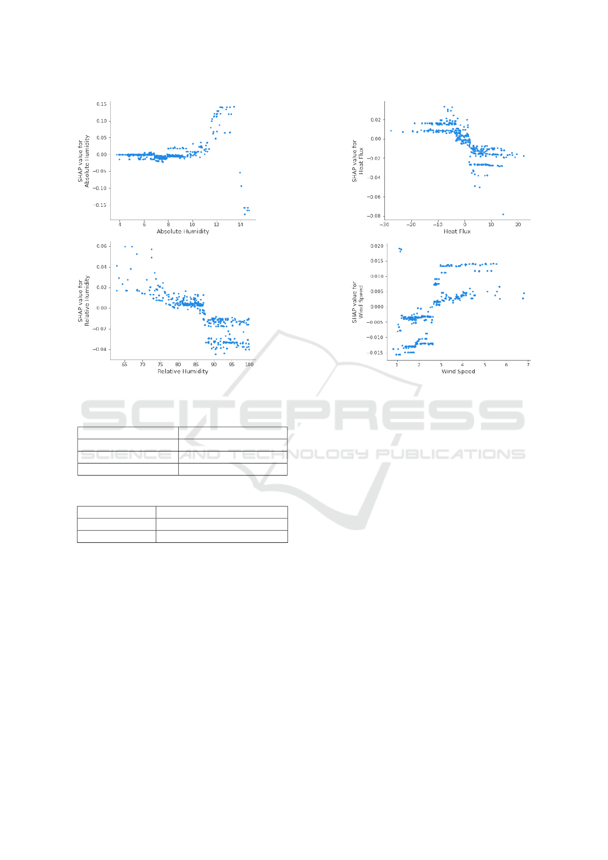
Figure 2: SHAP Feature Dependence Plot.

Table 1: Grid Search Cross Validation Parameters.

Parameter Values

Max depth 3, 6, 9, 12

Number of estimators 100, 200, 300, 400, 500

Learning rate 0.005, 0.015, 0.01, 0.1

Table 2: Keras Tuner Hyperparameters.

Hyperparameter Values

Number of units 16, 32, 64, 128

Learning rate 0.0003, 0.0001, ..., 0.03, 0.01

the performance of the best variant of each model on

two external sites for the year 2019: Chinmey Mead-

ows and Chobham. The two test sets were further di-

vided into three test subsets that covered the months

of January through April, May through August, and

September through December, respectively. Table 3

summarizes these results.

These results show that XG outperforms LSTM in

this prediction scenario while being less time consum-

ing. In comparison to 0.4722, 0.4746, and 0.6872 for

LSTM, the best performing variant of XG has MSE,

MAE, and RMSE of 0.3940, 0.4659, and 0.6277,

respectively. Figure 3 depicts the evolution of ac-

tual and predicted potential evapotranspiration on test

sites. These ﬁndings are consistent with those of

(Chakraborty et al., 2021), in which the authors state

that eXtreme Gradient Boosting can be more effective

than Long Short-Term Memory in predicting time-

series tabular data. Furthermore, the XG model devel-

oped in this study outperforms the hybrid deep learn-

ing model developed in (Xing et al., 2022), with RM-

SEs of 0.6277 and 0.651, respectively, despite using

signiﬁcantly less data.

The SHAP summary plot, shown in Figure 4 plot,

provides a global explanation of the XG model by

highlighting the importance of each feature as well

as its effect on the model’s outputs. According to the

ﬁgure, the top ﬁve contributing features to the model

are: net radiation, air temperature, heat ﬂux, air pres-

sure and relative humidity. While features such as net

radiation and air temperature have a positive overall

impact on the model’s output, the likes of heat ﬂux

and relative humidity have a negative impact. In other

words, low values of the ﬁrst two features (net radia-

tion and air temperature) are associated with low po-

tential evapotranspiration, whereas low values of the

last two (heat ﬂux and relative humidity) are associ-

ated with high potential evapotranspiration. This ex-

planation is critical because it demonstrates that the

model is correctly learning the dynamics of evapo-

transpiration. For example, it learned that high air

temperature lead to higher water loss. This is be-

cause high temperatures increase plant transpiration.

High relative humidity, on the other hand, indicates

Explainable Machine Learning for Evapotranspiration Prediction

101

Table 3: Results of XG on evaluation sites.

Site Data Coverage MSE MAE RMSE

Balruderry

January to April 0.2094 0.3358 0.4576

May to August 0.7937 0.7590 0.8909

September to December 0.1722 0.2963 0.4150

Chimney Meadows

January to April 0.2480 0.3615 0.4980

May to August 1.1066 0.8670 1.0519

September to December 0.2591 0.3695 0.5091

Chobham

January to April 0.3905 0.4640 0.6249

May to August 1.5314 1.0236 1.2375

September to December 0.3084 0.4197 0.5553

Figure 3: Actual vs XG Predicted Potential Evapotranspira-

tion.

the presence of a certain amount of water, leading to

a lower evapotranspiration value. As a result, XG, de-

spite being a black-box model, successfully captured

the fundamental principles of evapotranspiration.

Figure 4: SHAP Summary Plot of XG Model.

Furthermore, as shown in Figure 4, relative hu-

midity, heat ﬂux, and wind speed have the least inﬂu-

ence on the model’s predictions. Additionally, wind

speed feature seems not to be discriminatory enough

for the model as there is not a clear indication of its

overall impact on the predictions. Figure 2 gives fur-

ther detail about these features’ impact on evapotran-

spiration. It depicts the dependence plot of each fea-

ture with the target feature (potential evapotranspira-

tion). We can observe that most values of relative hu-

midity, wind speed and heat ﬂux have near to no im-

pact on the model as the corresponding shapley val-

ues turn around zero. This might indicate that these

features could be ignored for this particular predic-

tion. For this purpose, we retrained the model with-

out these two features to see how the model’s per-

formance changed. There was no discernible perfor-

mance loss, as we obtained MSE, MAE, and RMSE

values of 0.3777, 0.4512, and 0.6146 in comparison

to 0.3809, 0.4573, and 0.6171. Rather, we can notice

a slight improvement in model’s performance. As a

result, we achieved slightly better results while signif-

icantly simplifying the model and speeding up com-

putation.

Additionally, the test set’s subdivision allowed

us to identify the time frame with the highest er-

ror rate. The highest prediction errors (MSE, MAE,

and RMSE), as shown in Table 3, are encountered

between May and August. We will concentrate on

this subset of data to eventually provide additional

insights into the model’s learning abilities. For this

purpose, we provide model explanations using SHAP

collective force plot for data ranging from May to Au-

gust as illustrated in Figure 5.

The ﬁgure shows that the high values of Net Ra-

diation have the greatest inﬂuence on the majority of

the model’s decisions. As a result of the high Net

Radiation values observed between May and August,

the model is forecasting high evapotranspiration val-

ues. Because a large net radiation value from only the

past day might not be enough, we took into account

some past net radiation values instead. As a result, the

ICINCO 2023 - 20th International Conference on Informatics in Control, Automation and Robotics

102

Figure 5: SHAP Collective Force Plot from May to August.

model performed better, with MSE, MAE, and RMSE

values of 0.3578, 0.4409, and 0.5982, respectively.

Finally, Figure 6 shows local explanations for a

speciﬁc model’s prediction. Such information pre-

vents a model prediction from being used blindly be-

cause it explains why this particular instance was pre-

dicted. The ﬁgure, for example, shows that the model

was able to set thresholds for each parameter and

make decisions based on them. For example, air pres-

sure has a 0.07 positive impact on the prediction. A

positive inﬂuence raises the prediction value. The re-

maining features, on the other hand, had a negative

impact on the prediction. As a result, this can assist in

comprehending the internal process of the developed

model and, eventually, avoid erroneous prediction.

Figure 6: LIME explanations.

5 CONCLUSION

The present study proposed two machine learning

models to effectively predict potential evapotranspira-

tion. The study ﬁrst compared a deep learning LSTM

model with an extreme gradient boosting model. Al-

though the LSTM architecture has been initally de-

signed to deal with sequential data, our study demon-

strated that XG can outperform it. As a result, the

study established the suitability of such a model to

tabular time series data.

Next, because XG was the best-performing model,

we explained what and how the model learned from

data. Consequently, this study provided two types of

explanations: global and local. Global model expla-

nations using SHAP enabled us to recursively reﬁne

the model’s learning ability. As a result, we demon-

strated how explaining opaque models can aid in their

performance improvement. Local explanations using

LIME, on the other hand, were provided for some spe-

ciﬁc instances. These details help explaining why the

model made a particular prediction. In conclusion,

this study proposed an efﬁcient, explainable machine

learning model for predicting potential evapotranspi-

ration.

ACKNOWLEDGEMENTS

The work is carried out in the frame of the PREC-

IMED project that is funded under the PRIMA Pro-

gramme. PRIMA is an Art.185 initiative supported

and co-funded under Horizon 2020, the European

Union’s Programme for Research and Innovation.

(project application number: 155331/I4/19.09.18).

REFERENCES

Adeyemi, O., Grove, I., Peets, S., Domun, Y., and Nor-

ton, T. (2018). Dynamic Neural Network Mod-

elling of Soil Moisture Content for Predictive Irriga-

tion Scheduling. Sensors, 18(10):3408. Number: 10

Publisher: Multidisciplinary Digital Publishing Insti-

tute.

Barredo Arrieta, A., D

ıaz-Rodr

ıguez, N., Del Ser, J., Ben-

netot, A., Tabik, S., Barbado, A., Garcia, S., Gil-

Lopez, S., Molina, D., Benjamins, R., Chatila, R., and

Herrera, F. (2020). Explainable Artiﬁcial Intelligence

(XAI): Concepts, taxonomies, opportunities and chal-

lenges toward responsible AI. Information Fusion,

58:82–115.

Explainable Machine Learning for Evapotranspiration Prediction

103

Ben Abdallah, E., Grati, R., and Boukadi, K. (2022). A

machine learning-based approach for smart agricul-

ture via stacking-based ensemble learning and feature

selection methods. In 2022 18th International Con-

ference on Intelligent Environments (IE), pages 1–8.

ISSN: 2472-7571.

Ben Abdallah, E., Grati, R., and Boukadi, K. (2023). To-

wards an explainable irrigation scheduling approach

by predicting soil moisture and evapotranspiration via

multi-target regression. Journal of Ambient Intelli-

gence and Smart Environments, 15:89–110.

Chakraborty, D., Bas¸a

gao

glu, H., and Winterle, J. (2021).

Interpretable vs. noninterpretable machine learning

models for data-driven hydro-climatological pro-

cess modeling. Expert Systems with Applications,

170:114498.

Di Bucchianico, A. (2008). Coefﬁcient of Determination

(R2). John Wiley and Sons, Ltd.

Fereres, E. and Garc

ıa-Vila, M. (2018). Irrigation Man-

agement for Efﬁcient Crop Production. In Meyers,

R. A., editor, Encyclopedia of Sustainability Science

and Technology, pages 1–17. Springer, New York, NY.

Ghosal, S., Blystone, D., Singh, A. K., Ganapathysubrama-

nian, B., Singh, A., and Sarkar, S. (2018). An ex-

plainable deep machine vision framework for plant

stress phenotyping. Proceedings of the National

Academy of Sciences of the United States of America,

115(18):4613–4618. Place: Washington Publisher:

Natl Acad Sciences WOS:000431119600044.

Goap, A., Sharma, D., Shukla, A. K., and Rama Krishna,

C. (2018). An IoT based smart irrigation management

system using Machine learning and open source tech-

nologies. Computers and Electronics in Agriculture,

155:41–49.

Goldstein, A., Fink, L., Meitin, A., Bohadana, S., Luten-

berg, O., and Ravid, G. (2018). Applying machine

learning on sensor data for irrigation recommenda-

tions: revealing the agronomist’s tacit knowledge.

Precision Agriculture, 19(3):421–444.

Hochreiter, S. and Schmidhuber, J. (1997). Long Short-

Term Memory. Neural Computation, 9(8):1735–1780.

Jimenez, A.-F., Ortiz, B. V., Bondesan, L., Morata, G., and

Damianidis, D. (2021). Long Short-Term Memory

Neural Network for irrigation management: a case

study from Southern Alabama, USA. Precision Agri-

culture, 22(2):475–492.

Kon

e, B. A. T., Grati, R., Bouaziz, B., and Boukadi, K.

(2023). A new long short-term memory based ap-

proach for soil moisture prediction. Journal of Am-

bient Intelligence and Smart Environments, 15:255–

268.

Liakos, K. G., Busato, P., Moshou, D., Pearson, S., and

Bochtis, D. (2018). Machine Learning in Agriculture:

A Review. Sensors, 18(8):2674. Place: Basel Pub-

lisher: Mdpi WOS:000445712400274.

Navarro-Hell

ın, H., Mart

ınez-del Rincon, J., Domingo-

Miguel, R., Soto-Valles, F., and Torres-S

anchez, R.

(2016). A decision support system for managing ir-

rigation in agriculture. Computers and Electronics in

Agriculture, 124:121–131.

Ras, G., Xie, N., Gerven, M. v., and Doran, D. (2022).

Explainable Deep Learning: A Field Guide for the

Uninitiated. Journal of Artiﬁcial Intelligence Re-

search, 73:329–396.

Ribeiro, M., Singh, S., and Guestrin, C. (2016). “Why

Should I Trust You?”: Explaining the Predictions of

Any Classiﬁer. In Proceedings of the 2016 Confer-

ence of the North American Chapter of the Associa-

tion for Computational Linguistics: Demonstrations,

pages 97–101, San Diego, California. Association for

Computational Linguistics.

Rima, G., Myriam, A., and Kouloud, B. (2023). Towards a

novel approach for smart agriculture predictability. In

Proceedings of the 18th International Conference on

Software Technologies , ICSOFT’23, pages 96–105,

Italy, Rome. SCITEPRESS - Science and Technology

Publications.

Sammut, C. and Webb, G. I., editors (2010). Encyclopedia

of Machine Learning. Springer US, Boston, MA.

Schmidhuber, J. (2015). Deep learning in neural networks:

An overview. Neural Networks, 61:85–117.

Stanley, S., Antoniou, V., Askquith-Ellis, A., Ball, L., Ben-

nett, E., Blake, J., Boorman, D., Brooks, M., Clarke,

M., Cooper, H., Cowan, N., Cumming, A., Evans, J.,

Farrand, P., Fry, M., Hitt, O., Lord, W., Morrison, R.,

Nash, G., Rylett, D., Scarlett, P., Swain, O., Szczykul-

ska, M., Thornton, J., Trill, E., Warwick, A., and Win-

terbourn, B. (2021). Daily and sub-daily hydrometeo-

rological and soil data (2013-2019) [COSMOS-UK].

Sutskever, I., Vinyals, O., and Le, Q. V. (2014). Sequence to

sequence learning with neural networks. In Proceed-

ings of the 27th International Conference on Neural

Information Processing Systems - Volume 2, NIPS’14,

pages 3104–3112, Montreal, Canada.

Valiant, L. (2014). Probably Approximately Correct. Basic

Books, New York, 1st edition edition.

Xing, L., Cui, N., Guo, L., Du, T., Gong, D., Zhan, C.,

Zhao, L., and Wu, Z. (2022). Estimating daily ref-

erence evapotranspiration using a novel hybrid deep

learning model. Journal of Hydrology, 614:128567.

Yuan, Q., Shen, H., Li, T., Li, Z., Li, S., Jiang, Y., Xu, H.,

Tan, W., Yang, Q., Wang, J., Gao, J., and Zhang, L.

(2020). Deep learning in environmental remote sens-

ing: Achievements and challenges. Remote Sensing of

Environment, 241:111716.

Zhuang, S., Wang, P., Jiang, B., and Li, M. (2020). Learned

features of leaf phenotype to monitor maize water sta-

tus in the ﬁelds. Computers and Electronics in Agri-

culture, 172:105347.

ICINCO 2023 - 20th International Conference on Informatics in Control, Automation and Robotics

104