Adaptive Direct Compensation of External Disturbances for MIMO
Linear Systems with State-Delay
Bui Van Huan
1 a
, Alexey A. Margun
1,2 b
, Artem S. Kremlev
1 c
and Dmitrii Dobriborsci
3 d
1
Department of Control Systems and Robotics, ITMO University, St. Petersburg, Russia
2
IPME RAS, St. Petersburg, Russia
3
Deggendorf Institute of Technology, Dieter-Grlitz-Platz 1, 94469 Deggendorf, Germany
Keywords:
Compensation of External Disturbances, MIMO Systems, State-Delay, Full-Order Unknown Input Observer,
Observer of External Disturbance.
Abstract:
In the paper we propose a new method for compensation of external disturbances in MIMO linear systems
with unmeasured and delayed state vector. A state observer is used to estimate the state vector, which used
in another external disturbance observer. All these estimates are used in a control law to ensure asymptotic
convergence of the system outputs to zero and boundedness of all the closed loop signals. Proposed method
is based on the use of the internal model principle and the extended error adaptation algorithm. It is assumed
that the disturbance is the output of an autonomous linear generator with unknown parameters. To focus on
compensation of external disturbances, it is assumed that the system is stable and the delay is known constant.
The performance of the obtained results is confirmed using computer simulation in MATLAB Simulink.
1 INTRODUCTION
The paper considers the problem of external distur-
bance compensation with a stationary and bounded
amplitudes for a class of MIMO linear systems where
the state vector is unmeasured and delayed. Exter-
nal disturbance rejection for automatic systems is one
of the fundamental issues in control theory and has
received significant attention from researchers over
the years (Bodson and Douglas, 1996), (Nikiforov,
1996), (Marino et al., 2003). There are two methods
commonly used for disturbance compensation: direct
compensation and indirect compensation.
Indirect disturbance compensation is based on the
identification of disturbance parameters, including
amplitude, phase, frequency, and initial conditions
(Francis and Wonham, 1975), (Nguyen et al., 2022),
(Vlasov et al., 2018), (Vlasov et al., 2019). The ad-
vantage of this method is the independence of the
controller and the identifier. This enabling develop-
ers to apply various control strategies. However, this
method has a significant drawback, which is the re-
a
https://orcid.org/0000-0002-6563-1909
b
https://orcid.org/0000-0002-5333-0594
c
https://orcid.org/0000-0002-7024-3126
d
https://orcid.org/0000-0002-1091-7459
quirement for regressor persistent excitation. Failure
of this condition will result in incorrect identification
of disturbance parameters (Narendra, 1989).
Direct disturbance compensation is another ap-
proach to overcome the issue of persistent excitation
(Gerasimov et al., 2015), (Paramonov, 2018). This
approach employs the state variables or output signal
of the system to estimate the disturbance, which is
then utilized to synthesize a controller that achieves
the desired dynamics.
In practice most systems have a delay: an output
delay (due to the sensor) or an input delay (due to the
actuator) which adversely affects the performance of
the system. This factor even may cause system in-
stability. In (Fridman, 2014) author introduces vari-
ous studies on different aspects of delayed system and
control. In the (Chiasson and Loiseau, 2007) paper,
authors offer illustrations of delay systems applicable
to the domains of mechanical engineering, network
control, and communication.
Several studies (Banas and Vacroux, 1970),
(G
¨
ollmann et al., 2009), (Wu et al., 2019), (Sanz
et al., 2016) have been conducted to reduce the im-
pact of delay on the system. Combining the problem
of disturbance compensation and suppressing the ef-
fect of delay on the system makes the problem more
challenging (Pyrkin et al., 2015) (Paramonov, 2018),
236
Van Huan, B., Margun, A., Kremlev, A. and Dobriborsci, D.
Adaptive Direct Compensation of External Disturbances for MIMO Linear Systems with State-Delay.
DOI: 10.5220/0012256800003543
In Proceedings of the 20th International Conference on Informatics in Control, Automation and Robotics (ICINCO 2023) - Volume 2, pages 236-243
ISBN: 978-989-758-670-5; ISSN: 2184-2809
Copyright © 2023 by SCITEPRESS – Science and Technology Publications, Lda. Under CC license (CC BY-NC-ND 4.0)

(Van Huan Bui, 2022), especially when the delay and
the external disturbance are time varying (Liu et al.,
2022). However, the published researches and works
mainly focused on the delay in the control channel
(Gerasimov et al., 2015), (Paramonov, 2018). A few
works have considered systems with state delay (Frid-
man, 2014), (Gerasimov et al., 2019), (Kuperman and
Zhong, 2011) which commonly occur in fluid flow
models, communication networks and biological sys-
tems. To synthesize the control law and stabilize
the state delayed system a sliding mode control de-
sign using LMI was presented in (Gouaisbaut et al.,
2002). Dambrine M. and colleagues introduced feed-
back control of time-delayed systems with bounded
control and state in (Dambrine et al., 1995). Most of
the studies focus on SISO systems.
The presented method in the article offers the ad-
vantage of being able to compensate for external dis-
turbances on the system even when no information
about the disturbance is available (such as amplitude,
phase, or initial value). By only requiring knowledge
of the maximum number of harmonics, it is possi-
ble to provide a sufficiently large arbitrary value to
ensure the algorithm’s effectiveness. Secondly, the
direct disturbance compensation algorithm does not
require the identification of disturbance parameters,
thereby eliminating the requirement for persistent ex-
citation conditions. Finally, the method demonstrates
fast convergence to the system’s equilibrium state, re-
gardless of the arbitrarily chosen initial values.
Time-delay is a frequent occurrence in various
control systems, including aircraft, chemical or pro-
cess control systems. In many cases, delay can con-
tribute to instability, making the stability problem
of systems with delay significant both in theory and
practice. In order to analyze the problem in a more
visually accessible manner, we make the assumption
in this paper that the delay occurs only in the state
variable and consider its maximum value. In practice,
control systems may have input delays in the form of
multidelay, but the approach to solving the problem
remains essentially the same.
The paper is structured as follows: In Section I
a succinct problem description is provided. Section
II presents the mathematical problem statement with
several assumptions. Section III details the construc-
tion of a full-order state observer. Section IV focuses
on the development of an observer for external dis-
turbance. The synthesis of the control law and adap-
tation algorithm are presented in Section V. The sim-
ulation results in MATLAB are presented in Section
VI. Finally, Section VII provides our conclusions. To
demonstrate the performance of the proposed method
we conduct simulation in MATLAB Simulink.
2 PROBLEM STATEMENT
Let the mathematical model of a plant dynmics have
the form:
(
˙x(t) = A
1
x(t) + A
2
x(t − τ) + Bu(t) + E f (t)
y(t) = Cx(t)
(1)
where x(t), x(t −τ) ∈ R
n
are unmeasured state vector;
u(t) ∈ R
α
is the control signal vector; y(t) ∈ R
β
is
the system output; A
1
, A
2
, B,C, E are known constant
matrices with an appropriate dimension; f (t) ∈ R
γ
is
an unmeasured bounded external disturbance, where
γ is such that dim{E f (t)} = n.
The following assumptions are accepted:
Assumption 1. Matrix B has a full column rank and
matrix C has a full row rank.
Assumption 2. System (1) is stable, i.e. the roots
of the characteristic equation det(A
1
+ A
2
e
−τλ
−
λI
n×n
) = 0 lie in the left half-plane.
Assumption 3. The external disturbance vector f (t)
can be represented as the output of a linear au-
tonomous generator (Gerasimov et al., 2015):
(
˙w(t) = Γw(t)
f (t) = h
T
w(t)
where the matrices Γ, h
T
are unknown. The pair
(Γ, h
T
) is fully observable and the eigenvalues of the
Γ lie on the imaginary axis.
Assumption 2 is proposed to address the compen-
sation of external disturbances. In the case of an un-
stable system, it is possible to develop a control law:
u(t) = u
s
(t) + u
c
(t)
where u
c
(t) is compensating control component, u
s
(t)
is stabilizing control component. In practice, if dis-
turbance can be modeled as the output of a linear au-
tonomous generator, the proposed method can be used
for compensation. But in this paper for the conve-
nience of readers we assume that the external distur-
bance f (t) is a multi-harmonic signal. Without loss
of generality, assuming that the external disturbance
f (t) is the sum of harmonics in the form:
f (t) =
p
∑
j=0
R
j
sin(ω
j
t + φ
j
) + R
0 j
where p is maximum number of harmonics; R
j
are
unknown amplitudes; ω
j
are frequencies; φ
j
are
phases and R
0 j
are biases.
We must emphasize that from assumption 1 we
know the dimension of the disturbance and the maxi-
mum number of harmonics. Therefore, dimension of
the generator in assumption 3 is known. Assumption
Adaptive Direct Compensation of External Disturbances for MIMO Linear Systems with State-Delay
237

1 guarantees a MIMO system with a given number of
inputs and outputs. Assumption 3, the external dis-
turbance can be considered as the output of a linear
autonomous generator with unknown parameters but
with a known limited number of harmonics.
The goal of this paper is as follows: it is neces-
sary to construct a control law u(t) such that ensures
boundness of all signals in the closed loop system and
convergence of the output signal y(t) to zero when
time tends to infinity:
lim
t→∞
∥
y(t)
∥
= 0
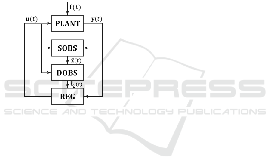
Figure 1 illustrates the closed system schematic of
the proposed approach.
Figure 1: The structure of the closed-loop system scheme
(SOBS is a full-order state observer, DOBS is an observer of
external disturbances, ˆx(t) is an estimate of the state vector,
ˆ
ξ
∑
(t) is an estimate of the regressor vector ξ
∑
(t).
3 CONSTRUCTION OF A
FULL-ORDER PLANT STATE
OBSERVER
To develop an external disturbance observer, it is im-
perative to create a full-order state observer due to the
unavailability of the state vector measurements. The
state observer developed in (Chen and Patton, 2012)
is utilized to construct a state observer with delay in
the form:





˙z(t) = Ez(t) + Fz(t − τ) + T Bu(t)
+L
1
y(t) + L
2
y(t − τ)
ˆx(t) = z(t) + Hy(t)
(2)
where z(t), z(t − τ) ∈ R
n
is a state vector of the full-
order observer; ˆx(t) ∈ R
n
is a state vector estimate;
E, F, T, L
1
, L
2
, H are constant observer’s matrices cho-
sen to satisfy the system of equations (3).
Proposition 1. The observer described by equation
(2) is considered a UIO (Unknown Input Observer)
for system (1) if and only if the following conditions
are holds:





































(I − HC)D = 0
T = I − HC
E = A
1
− HCA
1
− L
11
C
F = A
2
− HCA
2
− L
21
C
L
12
= EH
L
22
= FH
L
1
= L
11
+ L
12
L
2
= L
21
+ L
22
˙e
x
(t) = Ee(t) + Fe(t − τ) - is
asymptotically stable
(3)
where I is a unit matrix with an appropriate dimen-
sion, e
x
(t) = x(t)− ˆx(t), e
x
(t −τ) = x(t −τ)− ˆx(t −τ).
Proof. By differentiating e
x
(t) with (1) in time, we
obtain a dynamic model of observation error:
˙e
x
(t) = (A
1
− HCA
1
− L
11
C)e
x
(t) + [E
−(A
1
− HCA
1
− L
11
C)]z(t) + (A
2
− HCA
2
−L
21
C)e
x
(t − τ) + [F − (A
2
− HCA
2
−L
21
C)]z(t − τ) + [L
12
− (A
1
− HCA
1
− L
11
C)H]y(t)
+[T − (I − NC)]Bu(t) + [L
22
− (A
2
− HCA
2
−L
21
C)H]y(t − τ) + (HC − I)D f (t).
(4)
By substituting equation (3) into equation (4), we
get:
˙e
x
(t) = Ee(t) + Fe(t − τ)
Moreover, considering the final condition in the
proposition (1), it can be concluded that ˙e
x
(t)
t→∞
−−→ 0
for all initial conditions.
Proposition 2. The necessary and sufficient condition
for the system of equations (3) to have a solution are:
1. The rank of matrix CD is equal to the rank of ma-
trix D.
2. The matrix pair (C,
¯
A
1
) and (C,
¯
A
2
)
are detectable. where
¯
A
1
= A
1
−
D[(CD)
T
CD]
−1
(CD)
T
CA
1
and
¯
A
2
=
A
2
− D[(CD)
T
CD]
−1
(CD)
T
CA
2
.
Proof. The system of equations (3) has a solution if
and only if the equation (HC − I)D = 0 has a solu-
tion, which can be represented as HCD = D or alter-
natively (CD)
T
H
T
= D
T
. Matrix D
T
is a member of
the spectral space of matrix (CD)
T
, resulting in:
rank(D
T
) ⩽ rank((CD)
T
) ⇒ rank(D) ⩽ rank(CD)
ICINCO 2023 - 20th International Conference on Informatics in Control, Automation and Robotics
238

On the other hand,
rank(CD) ⩽ min{rank(C), rank(D)} ⩽ rank(D)
It is evident that the solution H =
D[(CD)
T
CD]
−1
(CD)
T
exists if and only if
rank(CD) = rank(D). It follows that:
E = A
1
− HCA
1
− L
11
C =
¯
A
1
− L
11
C
F = A
2
− HCA
2
− L
21
C =
¯
A
2
− L
21
C
according to condition (3) the matrix pair (C,
¯
A
1
) and
(C,
¯
A
2
) are detectable, which allows to choose the ma-
trix L
11
, L
21
such that ˙e
x
(t)
t→∞
−−→ 0, i.e. ˆx(t)
t→∞
−−→
x(t).
Consider Lyapunov function in the form:
V (e,t) = e
T
(t)Pe(t) +
t
Z
t−τ
e
T
(s)Qe(s)ds
where P and Q are two symmetric positive definite
matrices. The derivative of the Lyapunov function
with respect to time can be denoted as:
˙
V = e
T
(t)[E
T
P + PE + Q]e(t) + e
T
(t)PFe(t − τ)
+e
T
(t − τ)F
T
Pe(t) − e
T
(t − τ)Qe
T
(t − τ),
˙
V =

e
T
(t) e
T
(t − τ)

W

e(t)
e(t − τ)

.
where W =

E
T
P + PE + Q PF
F
T
P −Q

. In order to
˙
V < 0 matrix W must be negative.
Remark 1. To determine the matrices E and F that
satisfy the final condition of (3), one can utilize the
LTI toolbox in MATLAB. This will enable us to obtain
the matrices L
1
and L
2
.
Remark 2. If the matrix D does not have a full col-
umn rank, we can break the matrix D into D = D
1
D
2
.
Where D
1
has a full column rank and D
2
f (t) is con-
sidered as a new external disturbance.
4 CONSTRUCTION OF AN
EXTERNAL DISTURBANCE
OBSERVER
4.1 Parameterization of External
Disturbances
The output of an autonomous linear generator (Niki-
forov, 1996), (Gerasimov et al., 2015) is utilized to
represent the external disturbances:
(
˙
ξ(t) = G
∑
ξ
∑
(t) + L
∑
f (t)
f (t) = θ
T
∑
ξ
∑
(t)
(5)
where ξ
∑
(t) =

ξ
1
ξ
2
. . . ξ
q

T
∈ R
q
is a regres-
sor, G
∑
=




G
1
0 0 0
0 G
2
0 0
0 0
.
.
.
0
0 0 0 G
γ




, G
i
are Hurwitz ma-
trices; L
∑
=




L
1
0 0 0
0 L
2
0 0
0 0
.
.
.
0
0 0 0 L
γ




, L
i
are constant vec-
tors; θ
T
∑
∈ R
γ×q
is a vector of unknown constant pa-
rameters that depend on the disturbance parameters.
The pairs(G
i
, L
i
)are chosen arbitrarily to ensure that
each pair (G
i
, L
i
) is fully controllable.
4.2 An External Disturbance Observer
Base on the disturbance observer presented in (Niki-
forov, 1996), we propose a modified observer:





ˆ
ξ
Σ
(t) = ϕ
Σ
(t) + Q
Σ
x(t)
˙
ϕ
Σ
(t) = G
Σ
[ϕ
Σ
(t) + Qx(t)] − Q
Σ
A
1
x(t)
−Q
Σ
A
2
x(t − τ) − Q
Σ
Bu(t)
(6)
where
ˆ
ξ
∑
(t) =

ˆ
ξ
1
ˆ
ξ
2
. . .
ˆ
ξ
q

T
∈ R
q
is an esti-
mate of vector ξ
∑
(t); ϕ
∑
(t) =

ϕ
1
ϕ
2
. . . ϕ
q

T
∈
R
q
is an auxiliary vector used in the disturbance ob-
server; matrix Q
∑
=

Q
1
Q
2
. . . Q
γ

T
∈ R
q×n
satisfies:
Q
i
D = L
0i
where i = 1, γ is the number of the observer part cor-
responding to the external disturbance and the matrix
L
0i
:
L
0i
= [0
qi
, . . . , 0
qi
, L
i
, 0
qi
, . . . , 0
qi
]
where vector L
i
as the i − th column, and 0
qi
is the
q
i
-dimensional zero vector. This means that:
L
∑
= [
L
01
L
02
. . . L
0γ
]
T
Here e
ξ
(t) = ξ
∑
(t)−
ˆ
ξ
∑
(t) denotes the observation er-
ror. The time derivative of e
ξ
(t) with respect to (5)
and (6) can be expressed as:
˙e
ξ
(t) = G
∑
e
ξ
(t) + (L
∑
− N
∑
E)
|
{z }
0
f (t)
According to the assumption the matrix G
∑
is Hur-
witz. This implies that the observation error e
ξ
asymptotically converges zero. This is equivalent to
ˆ
ξ
∑
(t)
t→∞
−−→ ξ
∑
(t).
Furthermore, by solving equation (5), we obtain:
˙
ξ
∑
(t) = (G
∑
+ L
∑
θ
T
∑
)ξ
∑
(t)
⇒ ξ
∑
(t − τ) = P
−1
ξ
∑
(t)
Adaptive Direct Compensation of External Disturbances for MIMO Linear Systems with State-Delay
239

where P = exp(G
∑
+L
∑
θ
T
∑
) with the initial values set
to zero.
As a result, the external disturbance can be repre-
sented as:
f (t) = θ
T
∑
ˆ
ξ
∑
(t) + υ
where υ is an exponentially decaying function.
5 SYNTHESIS OF THE CONTROL
LAW AND ADAPTATION
ALGORITHM
To compensate external disturbances we create a con-
troller based on the research (Marino and Tomei,
2003). By utilizing the transformation matrix J we
convert the external disturbance coordinates into the
coordinate frame of the plant. The parametric track-
ing error of the plant state is then expressed as:
e(t) = x(t) − Jξ
∑
(t) (7)
Upon taking the derivative of equation (7) and taking
into account equations (1) and (5), we can obtain the
error dynamics:
˙e(t) = A
1
e(t) + A
2
e(t − τ) + [A
1
J + A
2
MP
−1
−J(Q
∑
+ L
∑
θ
∑
) + Dθ
T
∑
]ξ
∑
(t) + Bu(t)
and the output signal:
y(t) = C
T
e(t) +C
T
Jξ
∑
(t)
There always exists a pair of matrices J and ψ that is
a solution of the following system of equations:
(
A
1
J + A
2
JP
−1
− J(Q
∑
+ L
∑
θ
T
∑
) = Bψ
T
∑
− Dθ
T
∑
C
T
J = 0
The system of equations also known as the Francis or
regulator equations has at least one solution as stated
in (Francis and Wonham, 1975). The matrix ψ
T
∑
=
[ψ
1
, ψ
2
. . . ψ
α
]
T
∈ R
α×q
.
The dynamics of the error model can be obtained
in the following form:
(
˙e(t) = A
1
e(t) + A
2
e(t − τ) + B[ψ
T
∑
ξ
∑
(t) + u(t)]
y(t) = C
T
e(t)
(8)
Thus, the output signal vector can be reformulated as:
y(t) = W (s)[ψ
T
∑
ξ
∑
(t)] +W (s)[u(t)]
Alternatively, it can be written as:
y(t) = W (s)[ξ
T
∑
(t)]ψ
∑
+W (s)[u(t)] (9)
where W (s) = C
T
(sI − A
1
− A
2
e
−τs
)
−1
B
is matrix function. W (s)[ξ
T
∑
] =





W
11
(s)[ξ
T
∑
] W
12
(s)[ξ
T
∑
] ··· W
1α
(s)[ξ
T
∑
]
W
21
(s)[ξ
T
∑
] W
22
(s)[ξ
T
∑
] ··· W
2α
(s)[ξ
T
∑
]
.
.
.
.
.
.
.
.
.
.
.
.
W
β1
(s)[ξ
T
∑
] ·· · ·· · W
βα
(s)[ξ
T
∑
]





It should be noted that if ψ
T
∑
is a vector it can be
placed outside the brackets while maintaining the vec-
tor and its position unchanged in ψ
T
∑
W (s)[ξ
∑
]. In the
context of the paper, due to ψ
T
∑
being a matrix, it is
not permissible to exclude ψ
T
∑
from the transfer func-
tion in the conventional manner. To remove ψ
T
∑
from
the transfer function, the following procedure must be
executed:
W (s)[ψ
T
∑
ξ
∑
] = [W
i1
(s)[ξ
T
∑
] +W
i2
(s)[ξ
T
∑
]+
. . . +W
iα
(s)[ξ
T
∑
]]ψ
∑
Finally, we obtain
W (s)[ψ
T
∑
ξ
∑
] = W (s)[ξ
T
∑
]ψ
∑
From the disturbance observer (6)
ˆ
ξ
∑
(t) asymptoti-
cally converges to ξ
∑
(t), hence the control law for the
closed-loop system can be selected as:
u(t) = −
ˆ
ψ
T
∑
ˆ
ξ
∑
(t). (10)
5.1 Gradient Algorithm of Adaptation
We define the swapping term:
ς = W (s)[
ˆ
ψ
T
∑
ˆ
ξ
∑
] −W (s)[
ˆ
ξ
T
∑
]
ˆ
ψ
∑
and the augmented error:
¯y = y + ς
Considering the characteristics of linear systems and
the constant value of ψ
∑
, we can deduce the follow-
ing.
¯y = W (s)[(ψ
∑
−
ˆ
ψ
∑
)
T
ˆ
ξ
∑
] +W (s)[
ˆ
ψ
T
∑
ˆ
ξ
∑
]
−W (s)[
ˆ
ξ
T
∑
]
ˆ
ψ
∑
+ υ
¯y = W (s)[(ψ
∑
−
ˆ
ψ
∑
)
T
ˆ
ξ
∑
] +W (s)[
ˆ
ψ
T
∑
ˆ
ξ
∑
] −
W (s)[
ˆ
ξ
T
∑
]
ˆ
ψ
∑
+ υ
The system output error can be obtained by utilizing
equations (8) and (9):
¯y(t) = y(t) −W (s)[u(t)] −W (s)[
ˆ
ξ
T
∑
(t)]
ˆ
ψ
∑
¯y(t) = W (s)[
ˆ
ξ
T
∑
(t)]
˜
ψ
∑
(11)
where
˜
ψ
T
∑
= ψ
T
∑
−
ˆ
ψ
T
∑
.
Based on equation (11), we can synthesize a stan-
dard adaptation algorithm:
˙
ˆ
ψ
∑
= µW (s)[
ˆ
ξ
T
∑
(t)] ¯y(t) (12)
with the adaptive coefficient µ > 0.
ICINCO 2023 - 20th International Conference on Informatics in Control, Automation and Robotics
240

Proposition 3. Let assumptions 1-3 hold. The control
law (10) combined with the observer (2), (6) and the
adaptation algorithm (12) ensures in the closed-loop
system (1):
1. The boundedness of all signals in the closed-loop
system.
2. Output signal lim
t→∞
∥
y(t)
∥
= 0.
Proof. Let us denote the gradient function of
ˆ
ψ
∑
as∇
¯
J(
ˆ
ψ
∑
) with cost function
¯
J(
ˆ
ψ
∑
) =
1
2
¯y
2
. The gra-
dient descent of
ˆ
ψ
∑
has the form:
˙
ˆ
ψ
∑
= −µ∇
¯
J(
ˆ
ψ
∑
)
Taking the derivative of
¯
J(
ˆ
ψ
∑
) with respect to
ˆ
ψ
∑
we
obtain:
∂
¯
J(
ˆ
ψ
∑
)
∂
ˆ
ψ
∑
= ¯y
∂ ¯y
∂
ˆ
ψ
∑
;
∂ ¯y
∂
ˆ
ψ
∑
= −W (s)[
ˆ
ξ
T
∑
(t)]
⇒
˙
ˆ
ψ
∑
= µW (s)[
ˆ
ξ
T
∑
] ¯y
From equation (12) derive:
˙
˜
ψ
∑
= −µ∆∆
T
˜
ψ
∑
(13)
where ∆ = W (s)[
ˆ
ξ
∑
(t)], ∆
T
= W (s)[
ˆ
ξ
T
∑
(t)].
Select function Lyapunov as follows:
V (
˜
ψ
∑
) =
1
2µ
˜
ψ
T
∑
˜
ψ
∑
Subsequently, taking the derivative of V (
˜
ψ
∑
) with re-
spect to time using equation (12) yields the following
form:
˙
V =
˜
ψ
T
∑
˙
˜
ψ
∑
= −
˜
ψ
T
∑
∆ ¯y = − ¯y
2
≤ 0
5.2 Adaptation Algorithm with
Memory Regressor Extension
Within this subsection, our proposal involves the uti-
lization of the adaptive algorithm MRE, which was
introduced in (Nikiforov and Gerasimov, 2022), to ac-
celerate the achievement of system equilibrium (12).
By utilizing the extended error method, we obtain:
ˆy(t) = y(t) +W (s)[
ˆ
ξ
T
∑
(t)]
ˆ
ψ
∑
⇒ ˆy(t) = W (s)[
ˆ
ξ
T
∑
(t)]ψ
∑
By multiplying both sides by ∆ and subsequently
applying the transfer function H(s)to both sides, we
obtain:
Y = Ωψ
∑
(14)
where H(s) =
1
αs+β
, α > 0 is asymptotically stable
and minimal phase transfer function; Y = H(s)[∆ ˆy];
Ω = H(s)[∆∆
T
].
Based on equation (14), we can synthesize an al-
ternative adaptation algorithm:
˙
ˆ
ψ
∑
= µ(Y − Ω
ˆ
ψ
∑
) (15)
with the adaptive coefficient µ > 0.
Proposition 4. Let assumptions 1-3 hold. The control
law (10) combined with the observer (2), (6) and the
adaptation algorithm (15) ensures in the closed-loop
system (1):
1. The boundedness of all signals in the closed-loop
system.
2. Output signal lim
t→∞
∥
y(t)
∥
= 0.
Proof. From equation (14) we can get an extended
output error:
ε
Y
= Y − Ω
ˆ
ψ
∑
(16)
Substituting (14) in (16) we obtain:
ε
Y
= Y − Ω
ˆ
ψ
∑
=
H(s)[∆∆
T
˜
ψ
∑
] + H(s)[∆∆
T
ˆ
ψ
∑
] − Ω
ˆ
ψ
∑
ε
Y
= Ω
˜
ψ
∑
Using the gradient descent algorithm for the cost
function
¯
J(
ˆ
ψ
∑
) =
1
2
|
ε
Y
(
ˆ
ψ
∑
)
|
we have:
˙
ˆ
ψ
∑
= −µ∇
¯
J(
ˆ
ψ
∑
) = −µε
Y
(
ˆ
ψ
∑
)
∂ε
Y
(
ˆ
ψ
∑
)
∂
ˆ
ψ
∑
= µΩ(Y − Ω
ˆ
ψ
∑
)
Now the parameter error of the closed-loop system
described by equation:
˙
˜
ψ
∑
= −µΩ
2
˜
ψ
∑
It is easy to see that if µ > 0 then
˜
ψ
∑
t→∞
−−→ 0. There-
fore, it can be concluded that if the control system
satisfies the abovementioned assumptions 1-3, then
given the conditions of system (1) and external dis-
turbances, the selection of the adaptation coefficient
µ > 0 guarantees the boundedness of all signals in the
closed-loop system and the attainment of the target
condition: lim
t→∞
∥
y(t)
∥
= 0
6 SIMULATION RESULTS
As stated above, the algorithm presented in the paper
can be effectively employed in diverse domains, in-
cluding chemical process control, the quadruple tank
benchmark, and linear manipulator systems. To sim-
plify the algorithm to make it easier for readers to un-
derstand, we considered a third-order system as an il-
lustrative example:

˙x(t) = A
1
x(t) + A
2
x(t − τ) + Bu(t) + D f (t)
y(t) = Cx(t)
Adaptive Direct Compensation of External Disturbances for MIMO Linear Systems with State-Delay
241

with matrices A
1
=


−1 1 0
0 −1 1
−4 −5 −6


, A
2
=


0 −1 0
0 0 0.5
0 0 0


, B =


2 0
1 0
0 1


, D =


−1 0
0 0
−1 1


, C =

1 0 0
0 1 2

and initial conditions x(0) = [1;−1; 0].
External disturbances f (t) =

5sin(t)
1 + 5 sin(2t)

are
described by the output of autonomous linear genera-
tors with matrices: G
1
=

0 1
−3 −4

, L
1
=

0
2

and
G
2
=


0 1 0
0 0 1
−6 −11 −6


, L
2
=


0
0
6


.
To design a full-order state observer (2),
the matrix was chosen as follows: L
11
=


2.778 −0.111
−1.333 0.333
0.889 0.444


, L
21
=


12.579 −1.618
16.049 −15.900
−16.379 15.660


,
E =


−12.579 1.618 3.237
−16.050 14.900 32.800
16.378 −15.160 −31.820


,
F =


−2.779 0.111 0.222
1.333 −0.333 −0.167
−0.900 −0.444 −1.139


.
An observer of the external disturbances (6) was
constructed using the following matrices: Q
1
=

0 0 0
−2 0 0

, Q
2
=


0 0 0
0 0 0
−6 0 6


.
Figure 2 shows the transients using the standard
adaptation algorithm (12) with an adaptation gain µ =
5: output signal vector y(t) (a); estimation errors of
the state vector e
x
(t) (b); estimates of the tunable pa-
rameter vector
ˆ
ψ
∑
(c); control signal vector u(t) (d).
Figure 2: Graphs of transients of the standard adaptation al-
gorithm (12) with adaptation coefficient µ = 5: output sig-
nal vector y(t) (a); estimation errors of the state vector e
x
(t)
(b); estimates of the tunable parameter vector
ˆ
ψ
∑
(c); con-
trol signal vector u(t) (d).
Figure 3 shows the transients of the alternative
adaptation algorithm (15) with H(s) =
1
s+1
and adap-
tation gain µ = 25: output signal vector y(t) (a); es-
timation errors of the state vector e
x
(t) (b); estimates
of the tunable parameter vector
ˆ
ψ
∑
(c); control signal
vector u(t) (d).
Figure 3: Graphs of transients of the standard adaptation
algorithm (15) with adaptation coefficient µ = 25: output
signal vector y(t) (a); estimation errors of the state vector
e
x
(t) (b); estimates of the tunable parameter vector
ˆ
ψ
∑
(c);
control signal vector u(t) (d).
The simulation results show that using the stan-
dard adaptation algorithm (12) leads to the long tran-
sient time. Alternative adaptation algorithm (15) pro-
vides significantly decreased transient time. After 5
seconds of simulation, the state vector of the plant
converges to the true value x(t), which allows us to
conclude that it works correctly. Analysis of simu-
lation results has proven the applicability of the pro-
posed method.
7 CONCLUSIONS
In this paper, a novel approach for compensation of
external unknown disturbances in linear MIMO sys-
tems with state delay has been proposed. The ap-
proach outperforms existing techniques in terms of
the time required for the system to attain equilibrium
state, which is relatively short (15s). However, the
main limitation of this method lies in the require-
ment of being able to manipulate the coefficient ma-
trix D = D
1
D
2
of disturbance such that the resulting
rank(CD) is equal to rank(D). The simulation re-
sults in the MATLAB environment have demonstrated
the effectiveness of this method. In the future, this
method could be further developed to address prob-
lems in uncertain and state-delayed systems, as well
as control channel delay.
ICINCO 2023 - 20th International Conference on Informatics in Control, Automation and Robotics
242

ACKNOWLEDGEMENTS
The study was supported by the Ministry of Science
and Higher Education of the Russian Federation, state
assignment No. 2019-0898.
REFERENCES
Banas, J. and Vacroux, A. (1970). Optimal piecewise con-
stant control of continuous time systems with time-
varying delay. Automatica, 6(6):809–811.
Bodson, M. and Douglas, S. C. (1996). Adaptive al-
gorithms for the rejection of sinusoidal disturbances
with unknown frequency. IFAC Proceedings Volumes,
29(1):5168–5173.
Chen, J. and Patton, R. J. (2012). Robust model-based fault
diagnosis for dynamic systems, volume 3. Springer
Science & Business Media.
Chiasson, J. and Loiseau, J. J. (2007). Applications of time
delay systems, volume 352. Springer.
Dambrine, M., Richard, J.-P., Borne, P., et al. (1995). Feed-
back control of time-delay systems with bounded con-
trol and state. Mathematical Problems in Engineering,
1(1):77–87.
Francis, B. A. and Wonham, W. M. (1975). The inter-
nal model principle for linear multivariable regulators.
Applied mathematics and optimization, 2(2):170–194.
Fridman, E. (2014). Introduction to time-delay systems:
Analysis and control. Springer.
Gerasimov, D. N., Nikiforov, V. O., and Paramonov,
A. V. (2015). Adaptive disturbance compensation
in delayed linear systems: internal model approach.
In 2015 IEEE Conference on Control Applications
(CCA), pages 1692–1696. IEEE.
Gerasimov, D. N., Nikiforov, V. O., and Paramonov,
Alexei V, M. A. (2019). Adaptive tracking of mul-
tiharmonic signal in linear system with state delay.
Journal of Instrument Engineering, 62(9):772–781.
G
¨
ollmann, L., Kern, D., and Maurer, H. (2009). Optimal
control problems with delays in state and control vari-
ables subject to mixed control–state constraints. Op-
timal Control Applications and Methods, 30(4):341–
365.
Gouaisbaut, F., Dambrine, M., and Richard, J.-P. (2002).
Robust control of delay systems: a sliding mode
control design via lmi. Systems & control letters,
46(4):219–230.
Kuperman, A. and Zhong, Q.-C. (2011). Robust control
of uncertain nonlinear systems with state delays based
on an uncertainty and disturbance estimator. Inter-
national Journal of Robust and Nonlinear Control,
21(1):79–92.
Liu, C., Loxton, R., Teo, K. L., and Wang, S. (2022). Opti-
mal state-delay control in nonlinear dynamic systems.
Automatica, 135:109981.
Marino, R., Santosuosso, G. L., and Tomei, P. (2003).
Robust adaptive compensation of biased sinusoidal
disturbances with unknown frequency. Automatica,
39(10):1755–1761.
Marino, R. and Tomei, P. (2003). Output regulation for lin-
ear systems via adaptive internal model. IEEE Trans-
actions on Automatic Control, 48(12):2199–2202.
Narendra, K. S. (1989). Annaswamy. stable adaptive sys-
tems. Information And System Sciences. Prentice-
Hall.
Nguyen, T. K., Vlasov, S. M., Skobeleva, A. V., and Pyrkin,
A. A. (2022). Adaptive parameter estimation of de-
terministic signals. In 2022 8th International Confer-
ence on Control, Decision and Information Technolo-
gies (CoDIT), volume 1, pages 1291–1296. IEEE.
Nikiforov, V. (1996). Adaptive servocompensation of
input disturbances. IFAC Proceedings Volumes,
29(1):5114–5119.
Nikiforov, V. and Gerasimov, D. (2022). Adaptive regu-
lation: reference tracking and disturbance rejection,
volume 491. Springer Nature.
Paramonov, A. (2018). Adaptive robust disturbance com-
pensation in linear systems with delay. Nauchno-
Tekhnicheskii Vestnik Informatsionnykh Tekhnologii,
Mekhaniki i Optiki, 18(3):384.
Pyrkin, A. A., Bobtsov, A. A., Nikiforov, V. O., Kolyubin,
S. A., Vedyakov, A. A., Borisov, O. I., and Gromov,
V. S. (2015). Compensation of polyharmonic distur-
bance of state and output of a linear plant with delay in
the control channel. Automation and Remote Control,
76:2124–2142.
Sanz, R., Garcia, P., and Albertos, P. (2016). Enhanced
disturbance rejection for a predictor-based control of
lti systems with input delay. Automatica, 72:205–208.
Van Huan Bui, M. A. A. (2022). Compensation of out-
put external disturbances for a class of linear systems
with control delay. Journal Scientific and Technical
Of Information Technologies, Mechanics and Optics,
146(6):1072.
Vlasov, S. M., Kirsanova, A. S., Dobriborsci, D., Borisov,
O. I., Gromov, V. S., Pyrkin, A. A., Maltsev, M. V.,
and Semenev, A. N. (2018). Output adaptive con-
troller design for robotic vessel with parametric and
functional uncertainties. In 2018 26th Mediterranean
Conference on Control and Automation (MED), pages
547–552. IEEE.
Vlasov, S. M., Margun, A. A., Kirsanova, A. S., and Vakh-
vianova, P. (2019). Adaptive controller for uncertain
multi-agent system under disturbances. In ICINCO
(2), pages 198–205.
Wu, D., Bai, Y., and Yu, C. (2019). A new computational
approach for optimal control problems with multiple
time-delay. Automatica, 101:388–395.
Adaptive Direct Compensation of External Disturbances for MIMO Linear Systems with State-Delay
243