An Attention-Based Deep Generative Model for Anomaly Detection in

Industrial Control Systems

Mayra Macas

1,2 a

, Chunming Wu

1 b

and Walter Fuertes

2 c

College of Computer Science and Technology, Zhejiang University No. 38 Zheda Road, Hangzhou 310027, China

Department of Computer Science, Universidad de las Fuerzas Armadas ESPE, Av. General Rumi

nahui S/N,

P.O. Box 17-15-231B, Sangolqu

ı, Ecuador

Keywords:

Industrial Control Systems, Internet of Things, Deep Learning, Variational Autoencoder, Anomaly Detection,

Dynamic Threshold, CNN.

Abstract:

Anomaly detection is critical for the secure and reliable operation of industrial control systems. As our re-

liance on such complex cyber-physical systems grows, it becomes paramount to have automated methods

for detecting anomalies, preventing attacks, and responding intelligently. This paper presents a novel deep

generative model to meet this need. The proposed model follows a variational autoencoder architecture with

a convolutional encoder and decoder to extract features from both spatial and temporal dimensions. Addi-

tionally, we incorporate an attention mechanism that directs focus towards speciﬁc regions, enhancing the

representation of relevant features and improving anomaly detection accuracy. We also employ a dynamic

threshold approach leveraging the reconstruction probability and make our source code publicly available to

promote reproducibility and facilitate further research. Comprehensive experimental analysis is conducted on

data from all six stages of the Secure Water Treatment (SWaT) testbed, and the experimental results demon-

strate the superior performance of our approach compared to several state-of-the-art baseline techniques.

1 INTRODUCTION

Cyber-physical systems (CPSs) are incorporated,

complex systems that rely on unhindered communi-

cations between their cyber and physical parts. Re-

cently, they have established an instrumental role in

various sectors and have been adopted in many indus-

trial environments, such as electrical power grids, oil

reﬁneries, water treatment and distribution plants, and

public transportation systems (Macas et al., 2022). As

evidence, the respective market is expected to expand

by 9.7% per year, reaching up to US$9563 million

by 2025 (OrbisResearch, 2023). CPSs and the In-

ternet of Things (IoT) are interrelated concepts that

allow seamless communication between the physical

and digital worlds. At the same time, CPSs and IoT

also increase the likelihood of cybersecurity vulnera-

bilities and incidents due to the potential exploitations

of the heterogeneous communication systems in con-

trol of managing and controlling complex environ-

https://orcid.org/0000-0002-4328-6278

https://orcid.org/0000-0002-7538-0517

https://orcid.org/0000-0001-9427-5766

ments (Macas and Wu, 2019; Kravchik and Shabtai,

2022). Therefore, the capability of detecting sophisti-

cated cyber-attacks on the increasingly heterogeneous

nature of the CPSs, boosted by the arrival of IoT, has

become a crucial task.

In this work, it is assumed that the attackers aim

to change the physical behavior of their target, and

the primary objective is to defend the system beyond

the network level efﬁciently. Speciﬁcally, we consider

Industrial Control Systems (ICSs), which are a spe-

ciﬁc type of Cyber-Physical System that focuses on

regulating and monitoring industrial processes and in-

frastructure. They integrate physical components like

sensors, actuators, and machinery with computational

systems to enable efﬁcient and automated control of

manufacturing, power generation, and other industrial

operations.

The approaches that have recently been the focus

of attention employ supervised and unsupervised Ma-

chine Learning (ML) or Deep Learning (DL) models

to yield more intelligent and powerful techniques that

leverage big data to recognize anomalies and intru-

sions (Duo et al., 2022; Kravchik and Shabtai, 2018;

Goh et al., 2017b; Zhang et al., 2023). However,

566

Macas, M., Wu, C. and Fuertes, W.

An Attention-Based Deep Generative Model for Anomaly Detection in Industrial Control Systems.

DOI: 10.5220/0012264000003584

In Proceedings of the 19th International Conference on Web Information Systems and Technologies (WEBIST 2023), pages 566-577

ISBN: 978-989-758-672-9; ISSN: 2184-3252

even with ML/DL techniques, identifying anomalies

in the time series data describing the physical proper-

ties of the respective complex systems is a demanding

task. In particular, in order to develop models that can

automatically discover anomalies, one primary chal-

lenge is that only a small number of anomaly labels

are available in the historical data, which renders su-

pervised algorithms (Macas et al., 2022) impractical.

Consequently, this article proposes an unsu-

pervised anomaly detection method for ICSs built

upon an attention-based Convolutional Variational

Autoencoder (aCVAE). Speciﬁcally, we ﬁrst con-

struct statistical correlation matrices from the raw

time series data to characterize the system status

across different time steps. Then, the (convolutional)

encoder encodes a correlation matrix into a latent

representation roughly following a multidimensional

Gaussian distribution. The latent variable distribution

is represented by the mean and variance estimated by

the neural network. In addition, the attention mecha-

nism is introduced in the encoder as an attention mod-

ule to improve the spatial resolution of the correlation

matrices. On the other hand, the decoder performs

a series of reverse operations (i.e., dilated convolu-

tions) to reconstruct the correlation matrix from the

latent representation. The reconstruction probability

of aCVAE indicates the probability of the data orig-

inating from a speciﬁc latent variable sampled from

the approximate posterior distribution. Finally, this

reconstruction probability is leveraged to construct an

anomaly score to detect attacks.

The main contributions of this work can be sum-

marized as follows:

• We propose a new unsupervised reconstruction-

based method for detecting anomalies in mul-

tivariate time series data obtained from indus-

trial CPSs. The main component of the devised

methodology is a variational autoencoder with a

convolutional encoder and decoder named aC-

VAE. The latter adopts 3D-convolutions to extract

features from both spatial and temporal dimen-

sions effectively;

• We introduce an attention mechanism that guides

the proposed model to focus on speciﬁc regions

and enhances the representation of relevant fea-

tures;

• We use the reconstruction probability instead

of the commonly employed reconstruction error.

The reconstruction probability error measures the

probability of the reconstructed output given the

input rather than the difference between the input

and the reconstructed output;

• We adopt a dynamic threshold approach based on

an expected anomaly score estimator, enhancing

sensitivity and reducing false alarms;

• We make our source code publicly available

facilitate reproducibility and further research; and

• We perform comprehensive and comparative ex-

perimental analysis on data collected from all six

stages of the Secure Water Treatment (SWaT)

testbed (Goh et al., 2017a). The results demon-

strate the superior performance of the proposed

model over several state-of-the-art baseline tech-

niques.

2 RELATED WORK

Unsupervised learning techniques are used to un-

cover the underlying structure of unlabeled data.

These methods are popular in CPS intrusion detec-

tion (Macas et al., 2022) due to their simplicity and

ability to handle large datasets. For instance, an

SVM-based one-class (OC-SVM) classiﬁer and the

k-means clustering algorithm were used in (Maglaras

et al., 2020). K-means clustering served as a control

mechanism for the false positives generated by the

OC-SVM classiﬁer. However, the proposed algorithm

has some signiﬁcant drawbacks, such as the implicit

selection of a suitable kernel function that can vary

depending on the speciﬁc use case and its high com-

putational complexity. Furthermore, distance-based

clustering methods and the OC-SVM classiﬁer do not

consider the temporal dependencies between anoma-

lous data points (Almalawi et al., 2016), making them

susceptible to false positives and unsuitable for de-

tecting anomalies in complex systems.

Deep learning-based unsupervised anomaly de-

tection methods have recently gained signiﬁcant at-

tention. Goh et al. (Goh et al., 2017b) conducted a

study utilizing the deep LSTM-RNN model and Cu-

mulative Sum (CUSUM) to detect anomalies in the

ﬁrst stage of the SWAT dataset. The results indicated

that nine out of ten attacks were detected with only

four false positives. However, the stability of the re-

sults was not extensively discussed, which is regret-

table. Inoue et al. (Inoue et al., 2017) compared two

anomaly detection techniques: DNNs and OC-SVM.

According to their ﬁndings, DNNs had a precision of

98%, while OC-SVM had a precision of 92% across

all six stages of the SWaT dataset. It should be noted,

however, that the proposed architecture was rather

resource-demanding, complex, and challenging.

(Kravchik and Shabtai, 2018) conducted a study

on cyber-attack detection using a combination of 1D-

https://github.com/mmacas11/3Da-CVAE

An Attention-Based Deep Generative Model for Anomaly Detection in Industrial Control Systems

567

CNN and LSTM. Their approach successfully identi-

ﬁed attacks in all six stages of the SWAT dataset (Goh

et al., 2017a) with a precision rate of 91%. How-

ever, it was limited to detecting attacks in each stage

separately, without considering inter-stage dependen-

cies. In contrast, (Macas and Wu, 2019) developed

an attention-based Convolutional LSTM Encoder-

Decoder (ConvLSTM-ED) model, which analyzed

the entire SWaT testbed (Goh et al., 2017a). Their

approach achieved a precision rate of 96.0%, a re-

call rate of 81.5%, and an F1 score of 88.0%.

(Kravchik and Shabtai, 2022) employed 1D-CNN

and autoencoders to identify anomalies on the SWaT

dataset (Goh et al., 2017a). While their approach

yielded enhanced performance, it required manual

threshold setting for attack detection. On the other

hand, Xie et al. (Xie et al., 2020) proposed a hybrid ar-

chitecture utilizing CNN and RNN that achieved high

accuracy. However, they failed to consider that many

SWaT features have a different distribution in training

and testing data, which could result in false positives.

Overall, the above anomaly detectors share the

following two shortcomings within the context of

the problem we examine: (i) they need to consider

that data from sensors in real environments usually

contain noise—when that noise grows relatively se-

vere, it may hurt the generalization ability of tem-

poral prediction models, like those based on LSTMs

or RNNs (Malhotra et al., 2016); and (ii) the recon-

struction errors that are employed as anomaly scores

are difﬁcult to calculate if the data is heterogeneous.

In order to overcome these shortcomings, this pa-

per presents an efﬁcient anomaly detector for CPSs,

called aCVAE, which leverages an attention-based

Convolutional Variational Autoencoder to extract fea-

tures from both spatial and temporal dimensions ef-

fectively.

3 BACKGROUND

Herein, we brieﬂy overview the employed DL archi-

tectures.

3.1 Variational Autoencoder

The Variational Autoencoder (VAE) (Kingma and

Welling, 2014) is a directed probabilistic graphical

model whose posterior is approximated by a neural

network, forming an autoencoder-like architecture.

Given an input x, VAE applies an encoder (also known

as inference model) q

(z|x) to generate the latent vari-

able z that captures the variation in x. It uses a de-

coder p

(x|z) to approximate the observation given

the latent variable. The inference model represents

the approximate posterior using the mean µ and vari-

ance σ

calculated by q

(z|x), which is regularized to

be close to a Normal distribution. The prior p(z) is

chosen to be a standard Gaussian distribution. Given

the constraints of distribution on latent variables, the

complete objective function can be described as fol-

lows:

L (x|θ, φ) = −KL(q

(z|x)||p(z))

+ E

(z|x)



logp

(x|z)



, (1)

where KL(q

(z|x)||p(z)) is the Kullback-Leibler di-

vergence between the prior and the posterior. VAEs

have been applied successfully in different do-

mains. One such example is trafﬁc matrix estima-

tion (Kakkavas et al., 2021). Moreover, by employ-

ing statistical correlation matrices to characterize the

system status, VAEs can also be used for anomaly de-

tection in time series data (Xu et al., 2018; Chen et al.,

2020).

3.2 Convolutional Neural Networks

Convolutional neural networks (CNNs) use trainable

kernels to apply convolution operations on input im-

ages, generating spatial features that describe the tar-

get predictor (Goodfellow et al., 2016). The model

learns basic features in the initial layers and progres-

sively more complex representations in deeper lay-

ers. The output of a CNN is a set of feature maps

that can be directly used or passed on to a fully

connected layer for classiﬁcation or regression tasks.

A 3-dimensional CNN (3D-CNN) is a variation of

the typical 2-dimensional CNN (2D-CNN) that learns

spatio-temporal features by incorporating a third di-

mension. 3D convolutions are more effective than 2D

convolutions in capturing spatio-temporal patterns.

Even though CNNs are mostly used for image anal-

ysis, they have also proven successful in analyzing

multivariate time series data (Goodfellow et al., 2016;

Kravchik and Shabtai, 2022). 3D-CNNs are mainly

used for video analysis, but they have also been suc-

cessfully applied in other domains, such as network

trafﬁc forecasting (Guo et al., 2019) or predicting

damages in unmanned aerial vehicles (UAVs) (Varela

et al., 2022). Motivated by the above, in this work,

we introduce 3D convolutions to detect anomalies and

cyberattacks in multivariate time series obtained from

industrial CPSs.

3.3 Attention Mechanism

This research employs the 3D-Convolutional

Block Attention Module (3D-CBAM), inspired by

DMMLACS 2023 - 3rd International Special Session on Data Mining and Machine Learning Applications for Cyber Security

568

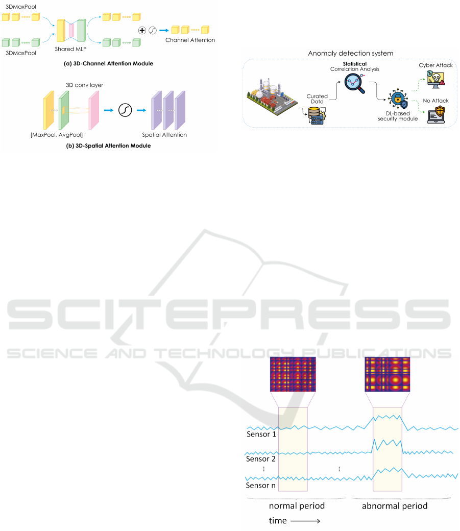
Figure 1: 3D-CBAM consists of (a) 3D-Channel Attention

Module and (b) 3D-Spatial Attention Module.

CBAM (Woo et al., 2018). As shown in Figure 1, 3D-

CBAM comprises two sub-modules: the 3D-channel

attention sub-module and the 3D-spatial attention

sub-module. In the former, 3D global maximum

pooling and 3D global average pooling decompose

the input into two vectors. Then, a Multi-Layer

Perceptron (MLP) generates two channel attention

maps, which are merged via element-wise sum-

mation. Finally, the 3D channel attention map is

generated using sigmoid activation. In the latter, the

maximum and average values over the input channel

are calculated and then concatenated. Finally, a

3D-convolution layer generates a spatial attention

map. These 3D-CBAM modules are placed between

the convolutional layers of the encoder in the aCVAE

model to help improve its accuracy by focusing on

essential features, inhibiting unnecessary elements,

and obtaining more representative points of interest.

4 FRAMEWORK AND

METHODOLOGY

In this section, we ﬁrst introduce the problem we

aim to study and then elaborate on the proposed

3D attention-based Convolutional Variational Au-

toencoder (aCVAE) in detail. Speciﬁcally, we ﬁrst

show how to generate correlation matrices from the

raw time series data to characterize the system status.

Next, the (convolutional) encoder encodes a correla-

tion matrix into a latent representation roughly fol-

lowing a multidimensional Gaussian distribution. In

addition, the attention mechanism is introduced in the

encoder as an attention module to improve the spatial

resolution of the correlation matrices. Then, the de-

coder performs a series of reverse operations (dilated

convolution being the reverse operation of convolu-

tion) to reconstruct the correlation matrix of the latent

representation. Finally, the reconstruction probabil-

ity is used as an anomaly score to detect anomalous

points. Figure 2 outlines the proposed framework.

Figure 2: Framework of the proposed anomaly detection

system.

4.1 Problem Statement

Consider m time series, X = (x

, x

, ··· , x

)

⊺

, x

, ··· , x

) ∈ R

m×T

, capturing the behavior of

m sensors over a period of time. Each time series,

= (x

, x

, ··· , x

)

⊺

∈ R

, represents the data col-

lected by the k

sensor for T time steps. At a given

time t, the vector x

= (x

, x

, ··· , x

)

⊺

∈ R

denotes

the corresponding values of all m time series. The

model aims to identify anomalous events at speciﬁc

time steps after T , assuming that the historical data

reﬂects normal system behavior, free of anomalies.

4.2 Statistical Correlation Analysis

Figure 3: Schematic representation of two system correla-

tion matrices (m×m) within normal and abnormal periods:

the correlation matrices differ because the system behavior

differs during normal and abnormal periods.

In order to detect abnormal behaviors in a system

that differ from legitimate ones, one can analyze its

statistical properties through a process called statis-

tical correlation analysis. This technique involves

comparing different pairs of time series to gain in-

An Attention-Based Deep Generative Model for Anomaly Detection in Industrial Control Systems

569

sight into the system’s status and has been exten-

sively studied (Macas and Wu, 2019). To repre-

sent the (inter)correlation between pairs of time se-

ries within a speciﬁc multivariate time series seg-

ment ranging from timestep t − w to t, an m ×

m correlation matrix M

is created by computing

the pairwise inner-product of every two component

time series segments. Figure. 3 provides two ex-

amples of such correlation matrices. More rigor-

ously, given a multivariate time series segment X

we calculate the correlation between the component

time series x



t−w

, x

t−w−1

, ··· , x



and x



t−w

, x

t−w−1

, ··· , x



using the following equation:

i j

∑

σ=0

t−σ

· x

t−σ

, (2)

with κ representing a rescaling factor (set equal to w

in the following). The correlation matrix M

∈ R

m×m

is utilized to capture the correlations in shape and

value scale between every pair of component time

series segments. This matrix is robust against input

noise, as turbulence within a time series has minimal

impact overall. In this work, we construct correla-

tion matrices at each time step with varying segment

lengths (w = 90, 150, 180), resulting in a total of three

matrices (s = 3) to describe the system’s state at dif-

ferent scales.

4.3 Attention-Based Convolutional

Variational Autoencoder (aCVAE)

In aCVAE, the input of the encoder is constructed

from the correlation matrix M

∈ R

m×m

and has di-

mensions (k, m, m, c) where k is the depth (i.e., the

number of frames/slices) in the 3D volume, m is the

height and the width of each frame, and c is the num-

ber of channels in each frame. The output is the mean

and variance parameters of the Gaussian probability

distribution of the latent variable z. The value of the

latent variable z is obtained by sampling from this

probability distribution. The encoder follows a 3D-

fully-convolutional network (FCN) architecture (Li,

2017) to process M

. It consists of four 3D con-

volution layers (e.g. spatial convolution over vol-

umes) (Long et al., 2015) and one fully connected

layer. Furthermore, we insert 3D-CBAM attention

modules (see Section 3.3) between the fully convo-

lution layers to focus and improve the spatial resolu-

tion of the correlation matrix. In particular, the atten-

tion process in the CBAM module can be summarized

as (Huang et al., 2020):

′

= F

) ⊗ M

and

′′

= F

′

) ⊗ M

′

(3)

where F

∈ R

1×1×1×c

is the channel attention map and

∈ R

k×m×m×1

is the spatio-temporal attention map.

The channel attention map and spatio-temporal atten-

tion map are calculated as follows:

) = σ(Conv3D(AvgPool(M

))+

Conv3D(MaxPool(M

))) and

′

) = σ(Conv3D(AvgPool(M

′

);MaxPool(M

′

)))

(4)

The input of the decoder is the latent representation

z obtained from the encoder, and the output is the

mean and variance of the posterior Gaussian proba-

bility distribution and the reconstructed

from the

latent variables. Like the encoder, the decoder is mod-

eled using a 3D-fully-convolutional network (FCN)

structure (Li, 2017). It consists of ﬁve transposed con-

volution layers and one fully connected layer. The de-

tailed structure of the encoder and decoder is shown

in Figure 4.

For all the convolution layers and transposed con-

volution layers in the encoder and decoder, the recti-

ﬁed linear activation function or ReLU (Goodfellow

et al., 2016), glorot uniform initializer (Goodfellow

et al., 2016), and batch normalization (Goodfellow

et al., 2016) with a decay of 0.9 are used. The acti-

vation function, weight initializer, and batch normal-

ization for the last fully connected layer are omitted.

Lastly, the dimension of the latent space is set to 100.

To converge the parameters θ and φ of the encoder

and decoder, the aCVAE is trained to maximize the

Evidence Lower Bound (ELBO), which can be ex-

pressed as the sum of two components: the recon-

struction term and the regularization term. The for-

mer is calculated as the reconstruction log-likelihood

of M

and the latter is the Kullback-Leibler (KL) di-

vergence between the learned posterior latent distri-

bution and a prior distribution, often a simple Gaus-

sian distribution. The Adam optimizer (Goodfellow

et al., 2016) is used for maximizing the ELBO during

training, which is computed by:

ELBO

|θ, φ) = −KL(q

(z|M

)||p(z))+

(z|M

)



logp

|z)



(5)

The reconstruction probability of aCVAE indi-

cates the probability of the data originating from a

speciﬁc latent variable sampled from the approxi-

mate posterior distribution. The anomaly score was

DMMLACS 2023 - 3rd International Special Session on Data Mining and Machine Learning Applications for Cyber Security

570

Figure 4: Architecture of the aCVAE with respect to an input of size 40 × 40 × 1.

set equal to one minus the reconstruction probabil-

ity, which is calculated by the Monte Carlo estimate

(z|M

)



logp

|z)



, the second term of the right-

hand side of Equation 5. Data points with anomaly

scores higher than threshold τ are identiﬁed as

anomalies, and those with anomaly scores lower

than τ are considered normal.

State-Based Thresholding

Drawing inspiration from (Park et al., 2018), we pro-

pose a dynamic threshold that adapts to the esti-

mated state of task execution. Reconstruction qual-

ity can vary depending on the execution’s state, and

sometimes, non-anomalous executions can have high

anomaly scores in certain states. By dynamically

adjusting the threshold, we can reduce false alarms

and improve sensitivity. In our problem formulation,

the state refers to the latent space representation of

observations, which the encoder of aCVAE can cal-

culate for each time step in a sequence of observa-

tions. Our approach involves training an expected

anomaly score estimator,

: z −→ s, by mapping

states Z and corresponding anomaly scores S from the

non-anomalous dataset. Speciﬁcally, we use a non-

parametric Bayesian approach called Gaussian Pro-

cess Regression (GPR) to map the multidimensional

inputs z ∈ Z to the scalar outputs s ∈ S employing a

radial basis function (RBF) kernel with noise. More-

over, a constant η is added to the expected score

to control sensitivity, thus forming the following dy-

namic state-based threshold: τ =

(z) + η.

5 EXPERIMENTAL ANALYSIS

In this section, we conduct extensive experiments to

answer the following research questions:

• RQ1: Can aCVAE outperform baseline methods

for anomaly detection in multivariate time series?

• RQ2: How does each component of aCVAE af-

fect its performance?

5.1 Experimental Setup

Dataset

The Secure Water Treatment (SWaT) testbed (Goh

et al., 2017a) is an invaluable resource for researchers

studying complex CPS environments. With data col-

lected from 51 sensors and actuators every second, the

Historian Server provides a wealth of information for

analysis. The SWaT dataset contains seven days of

normal operating conditions and four days of record-

ings, during which 36 attacks were carried out. These

attacks simulated a system already compromised by

attackers, who interfered with normal system opera-

tion and spoofed the system state to the PLCs, caus-

ing erroneous commands to be broadcast to the actu-

ators. The attacks were carried out by modifying the

network trafﬁc in the level 1 network, issuing false

SCADA commands, and spooﬁng the sensors’ values.

This dataset includes attacks that target a single stage

of the process and simultaneous attacks on different

stages.

An Attention-Based Deep Generative Model for Anomaly Detection in Industrial Control Systems

571

Data Pre-Processing

Considering that this study focuses on physical layer

attacks, we used the “Physical” subdirectory of the

SWaT dataset containing 51-time series (variables)

generated by sensors and actuators on a per-second

basis. The SWaT dataset was ﬁrst pre-processed by

discarding the data that did not help improve the de-

tection accuracy (e.g., the features with constant val-

ues), retaining 40 out of the original 51 features. The

resulting data were also normalized, so the range of

observed values lies in the interval [0, 1]. Among

the raw data, 495 000 records were collected under

normal conditions, and 449 919 were collected while

performing various cyber-attacks in the system. Our

experiments divide the dataset captured under normal

conditions into three subsets. In particular, we use the

ﬁrst 336 560 data points as the training set (N

nornal

);

the following 96 160 data points form the ﬁrst nor-

mal validation set (V

normal1

) that is used for early

stopping while training the proposed model and the

remaining 48 080 data points the second normal val-

idation set (V

normal2

), which is used for tuning the

hyper-parameters of the model and for determining

the threshold. Finally, the dataset containing anoma-

lies, denoted by A

abnornal

and comprising 449 919

points, is employed as the test set.

Baselines and Variants

To determine how well our proposed model works,

we compared it to six other baseline approaches that

are commonly used in similar situations. These ap-

proaches are well-known and respected for measuring

performance. Our goal was to identify the strengths

and weaknesses of our model and determine if it is

better than the other approaches for solving the prob-

lem at hand. Speciﬁcally, the considered approaches

include:

1) One-Class SVM (OC-SVM) (Inoue et al.,

2017) and 2) Isolation Forest (IF) (Cheng et al.,

2019), where the classiﬁcation models learn a de-

cision function and classify the test dataset as sim-

ilar or dissimilar to the training dataset;

3) Density-Based Local Outliers (LOF) (Al-

malawi et al., 2014) and 4) Gaussian Mix-

ture Model (GMM) (McLachlan and Rathnayake,

2014), which are density-based approaches as-

signing to each object of the test dataset a degree

of being an outlier;

5) Long Short-Term Memory-based Encoder De-

coder (LSTM-ED) (Malhotra et al., 2016) and 6)

Gated Recurrent Unit Encoder Decoder (GRU-

ED) (Dey and Salem, 2017), which are able to

capture and represent the training dataset’s tem-

poral dependencies.

The anomaly scores are computed similarly to (Mal-

hotra et al., 2016). Broadly speaking, to identify

anomalies in a test time series, we use reconstruc-

tion errors to calculate the likelihood of a point be-

ing anomalous. This is done through Maximum

Likelihood Estimation, which assigns each point an

anomaly score. The higher the score, the more likely

the point is anomalous.

Besides the aforementioned models, we consider

three aCVAE variants to justify the effectiveness of

each component of the complete model:

7) 2D-CVAE, where the 3D convolutional layers

are replaced by 2D convolutional layers and

8) 3D-CVAE, where the attention module is re-

moved.

9) A deterministic 3D convolutional autoencoder,

which is used to quantify the gains of using prob-

abilistic modeling via the variational autoencoder.

Evaluation Metrics

We measure the effectiveness of each method in de-

tecting anomalous events using precision (Prec), re-

call (Rec), and F

score (Sammut and Webb, 2016),

computed as follows:

Prec =

TP + FP

Rec =

TP + FN

, and

score =

2 · Prec · Rec

Prec + Rec

where TP, FP, TN and FN stand for true positives,

false positives, true negatives, and false negatives, re-

spectively. Each model’s ability to avoid False Posi-

tives is measured by Precision (Prec), the proportion

of correctly predicted positive instances out of all in-

stances predicted as positive. Recall (Rec) is also

known as sensitivity or True Positive Rate, and it mea-

sures the model’s ability to avoid False Negatives. It

is deﬁned as the proportion of correctly predicted pos-

itive instances out of all positive ones. Lastly, the

F1 score is a balanced measure of the model’s per-

formance, considering both False Positives and False

Negatives. It is calculated as the harmonic mean of

precision and recall.

To detect an anomaly, we leverage that the recon-

struction errors of anomalous data are expected to be

larger than those of normal data. The main idea is

that due to the training over normal historical data,

DMMLACS 2023 - 3rd International Special Session on Data Mining and Machine Learning Applications for Cyber Security

572

the employed generative model has learned “well” to

reconstruct the respective correlation matrices, i.e.,

the correlation matrices corresponding to normal op-

eration. Consequently, the model is expected to re-

construct similarly well any normal correlation ma-

trices during the testing phase. On the contrary, an

anomaly—deﬁned as an outlier or discrepancy—will

lead to a larger reconstruction error since the varia-

tional autoencoder has not learned to model it efﬁ-

ciently.

Finally, we use a summary metric called PRAUC

(Precision-Recall Area Under the Curve) (Brown and

Davis, 2006) to measure the classiﬁer’s overall perfor-

mance. This metric is calculated by quantifying the

trade-off between precision and recalls for different

classiﬁcation thresholds, as shown on the Precision-

Recall curve. We obtain a single scalar value rep-

resenting the model’s overall performance by calcu-

lating the area under this curve. A higher PRAUC

value indicates that the model performs better regard-

ing precision and recall.

Implementation Details

The proposed method and its variants, as well as

LSTM-ED, were implemented in Python 3.9.12

utilizing the TensorFlow framework version

2.12.0 (Abadi et al., 2016) and the Keras (Chol-

let et al., 2015) deep learning API. In particular, we

utilize the subclassing API to customize models by

subclassing the tf.keras.Model class. This allows

for greater control and ﬂexibility over the model’s

architecture and behavior compared to the sequential

or functional API. The constructor deﬁnes the layers

and operations that make up the model, while the

call method deﬁnes the model’s forward pass.

When inputs are passed to the model, this method

connects the layers and applies operations to the

inputs to deﬁne the computation graph of the model.

The standard Keras workﬂow compiles and trains the

model, specifying the loss function, optimizer, and

metrics. Finally, the predict method is used to make

predictions with the model.

We implemented the traditional baseline tech-

niques, namely OC-SVM, LOF, IF, and GMM, uti-

lizing Python version 3.9.12 in conjunction with the

Scikit-learn library (Pedregosa et al., 2011). Our ex-

perimentation took place on a Linux server equipped

with six virtual central processing units (vCPUs) and

15 gigabytes (GB) of RAM. This server setup ensured

ample computational capabilities for the efﬁcient ex-

ecution of our experiments.

5.2 Experimental Results

In order to answer the RQ1, we evaluate the models’

performance on the six stages of the SWaT dataset in

terms of precision (Pre), recall (Rec), and F1 score.

The experiments are repeated ﬁve times, and we re-

port the average results in Table 1 for comparison,

where the best overall scores are highlighted in bold

and the best baseline scores are indicated by dou-

ble underline and italics. It should be noted that the

baseline methods are evaluated over the raw time se-

ries data since they cannot work with multidimen-

sional (in our case, two-dimensional) data. We ob-

serve that the traditional models (i.e., OC-SVM, IF,

LOF, and GMM) perform worse than the deep predic-

tion models (i.e., LSTM-ED and GRU-ED), indicat-

ing that they cannot adequately handle the temporal

dependencies in the dataset. However, the approaches

based on LSTM and GRU have lower recall and F1

scores than deep models based on 3D convolutions.

Although LSTM and GRU can handle the temporal

dependencies in the data, they can not extract the fea-

tures from the spatial dimension. More concretely,

are unsuitable for simultaneously learning spatial and

temporal dependencies, contrary to approaches based

on 3D-CNNs.

The 3D-CAE and the aCVAE architectures yield

the largest precision when w = 90. However, the aC-

VAE model achieves the largest recall and F1 score

for all the employed window sizes. Hence, this ver-

iﬁes that the proposed 3D attention-based Convolu-

tional Variational Autoencoder (aCVAE) architecture

efﬁciently identiﬁes anomalies or outliers. Next, we

demonstrate how the performance of the aCVAE ap-

proach varies across the employed sequence window

lengths w = {90, 150, 180}. In particular, aCVAE

with w = {90, 150} has better precision than aCVAE

with w = 180, whereas aCVAE with w = 90 has bet-

ter recall and F1 rate compared to the other window

lengths. Figure 5 summarizes the evaluation met-

rics for the aCVAE model and its variants when the

window length equals 90. Furthermore, to provide

a detailed comparison, Figure 6 contrasts the perfor-

mance of aCVAE and the best baseline method, i.e.,

LSTM-ED, for the SWaT dataset. It is evident that the

anomaly score of LSTM-ED is not stable, resulting in

numerous false positives (blue points that are above

the threshold line) and false negatives (gray points

that are below the threshold line). In contrast, aCVAE

demonstrates better anomaly detection performance

with fewer misclassiﬁcations.

To answer the RQ2, Table 2 presents the perfor-

mance of the three variants of aCVAE architecture

(i.e., 3D-CAE, 2D-CVAE, and 3D-CVAE) in terms of

An Attention-Based Deep Generative Model for Anomaly Detection in Industrial Control Systems

573

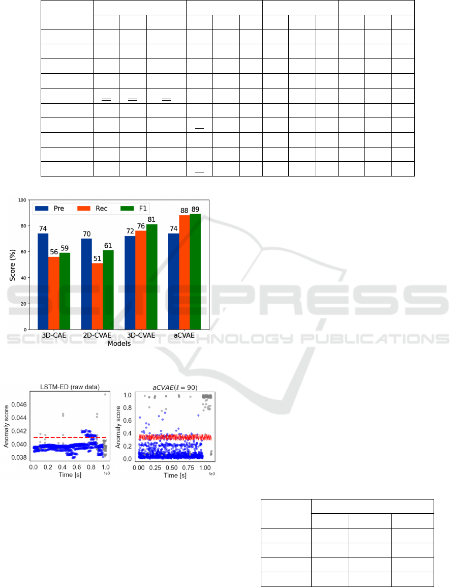
Table 1: Average anomaly detection results for all the considered methods and models.

Method

Raw time series data w = 90 w = 150 w = 180

Pre Rec F1 Pre Rec F1 Pre Rec F1 Pre Rec F1

OC-SVM 50 47 40 - - - - - - - - -

IF 65 60 55 - - - - - - - - -

LOF 67 55 57 - - - - - - - - -

GMM 70 50 60 - - - - - - - - -

LSTM-ED 71 59 72 - - - - - - - - -

GRU-ED 70 55 74 - - - - - - - - -

3D-CAE - - - 74 56 59 81 73 79 62 77 65

2D-CVAE - - - 70 51 61 72 68 74 67 79 72

3D-CVAE - - - 72 76 81 79 75 83 66 70 84

aCVAE - - - 74 88 89 80 76 88 70 82 87

Figure 5: The performance of different deep models when

w=90.

Figure 6: Representative illustration of anomaly detection.

The sections shaded in grey indicate periods of anomalies.

The red dashed line represents the threshold for detecting

anomalies in the SWaT dataset.

PRAUC, to indicate the impact and the signiﬁcance of

the various components of the proposed model. We

observe that the 3D convolutional layers improve the

performance of aCVAE. In particular, a 3D convolu-

tional layer uses a three-dimensional ﬁlter to perform

convolutions. The kernel can slide in three directions,

whereas a 2D CNN can slide only in two dimensions.

Within the context of this work, the third dimension

is time. Thus, the 3D convolutional layers are more

effective in learning meaningful spatio-temporal fea-

tures from the correlation matrices, contrary to 2D

convolutional layers, which cannot handle temporal

patterns.

Moreover, aCVAE outperforms 3D-CAE and 3D-

CVAE, which suggests that the 3D attention mecha-

nism incorporated between the 3D convolutional lay-

ers in the decoder can further improve anomaly de-

tection performance. Figure 7 provides a visual rep-

resentation of the ability of the methods mentioned

above to detect anomalies. It presents the PRAUC

of the different deep models over different window

lengths: (w = 90, 150, 180). As can be seen, aCVAE

outperforms the other deep learning models, generat-

ing higher PRAUC. In particular, the highest PRAUC

is achieved when the window length equals 90 (i.e.,

one minute and a half). Generally, the PRAUC of

deep models based on 3D convolutions decreases as

the window length increases. Thus, it is recom-

mended not to choose a large window length, given its

impact on performance and higher computation cost.

Table 2: PRAUC of the aCVAE model and its variants over

different window lengths.

Models

PRAUC

w = 90 w = 150 w = 180

3D-CAE 0.8123 0.7212 0.7589

2D-CVAE 0.6574 0.6841 0.6974

3D-CVAE 0.8379 0.8107 0.8002

aCVAE 0.9015 0.8801 0.8725

Figure 8 provides a visual representation of the

ability of the aCVAE, 3D-CAE, 2D-CVAE, and 3D-

DMMLACS 2023 - 3rd International Special Session on Data Mining and Machine Learning Applications for Cyber Security

574

Figure 7: Visual representation of PRAUC for aCVAE and

its variants over different windows sizes.

CVAE architectures to detect anomalies and the ef-

ﬁciency of the proposed dynamic threshold over a

speciﬁc testing period of 60 seconds. Note that the

anomalous execution originated from the SSSP attack

aiming to overﬂow the tank at P3. As can be seen, aC-

VAE can effectively detect the anomaly, which begins

in 43 seconds, contrary to 3D-CVAE, 2D-VAE, and

3D-CAE, which produce many false positives. Be-

sides, we can see that depending on the state of task

executions, reconstruction quality may vary. In other

words, anomaly scores in non-anomalous task execu-

tions can be high in certain states, so varying the dy-

namic state-based threshold according to the expected

anomaly score can reduce false alarms and improve

sensitivity.

Moreover, Figure 8 provides insights into the ad-

vantages of using the reconstruction probability in-

stead of a deterministic reconstruction error, com-

monly used in autoencoder-based anomaly detection

approaches (e.g., 3D-CAE). The ﬁrst one is that

the reconstruction probability does not require data-

speciﬁc detection thresholds since it is a probabilistic

measure. Using such a metric provides a more intu-

itive way of analyzing the results. The second one is

that the reconstruction probability considers the data’s

variability. Intuitively, anomalous data has higher

variance than normal data, and hence, the reconstruc-

tion probability is likely to be lower for anomalous

examples. Using the variability of data for anomaly

detection enriches the expressive power of the pro-

posed model compared to conventional autoencoders.

Even when normal and anomalous data can share the

same expected value, the variability is different and,

thus, provides an extra tool to distinguish anomalous

examples from normal ones.

The 3D-CBAM attention mechanism makes the

aCVAE more understandable, reliable, and efﬁcient.

Figure 8: Visualization of the anomaly scores over a test-

ing period of 60 s for aCVAE. The dashed curve represents

the dynamic state-based threshold, based on which the aC-

VAE performs anomaly detection: an anomaly is identiﬁed

when the current anomaly score is larger than the thresh-

old. The brown color represents the duration of the detected

anomaly.

Figure 9 illustrates how 3D-CBAM allows the aC-

VAE to weigh features by the level of importance for

detecting anomalous points. Speciﬁcally, 3D-CBAM

enables the model to identify the most relevant re-

gions in the correlation matrices. As shown in Fig-

ure 9, the correlation matrix that goes through the

convolution layer + 3D-CBAM is more accurate than

the one that goes through the vanilla convolutional

layers. This visualization demonstrates the feature

map for a speciﬁc input correlation matrix to observe

the detected and preserved input features.

Figure 9: Correlation matrix corresponding to SSSP attack

aiming to overﬂow the tank at P3 passed through the 3D

convolutional layer + 3D-CBAM and vanilla 3D convolu-

tional layer.

5.3 Discusion

We propose the 3D attention-based Convolutional

Variational Autoencoder or aCVAE for unsupervised

anomaly detection over industrial time series data.

We address the existing methods’ limitations: poor

An Attention-Based Deep Generative Model for Anomaly Detection in Industrial Control Systems

575

generalization to unseen anomaly patterns and using

supervised methods to learn a suitable threshold strat-

egy. For the latter, as the nature of the data pro-

duced by the CPSs continuously changes and insuf-

ﬁcient labeled data for each class are available, more

than supervised methods are needed. In aCVAE, the

stochastic latent variable is learned from spatial and

temporal dependencies of the correlation matrices,

making the reconstruction more generalized. A ro-

bust objective function is integrated into the mod-

els to avoid the contamination problem of the la-

tent space. Finally, an unsupervised dynamic-based

threshold-setting strategy is adopted, instead of the

traditional supervised ROC-based strategy, to achieve

better model performance. The reported experimental

results demonstrate that aCVAE can outperform state-

of-the-art baseline methods.

6 CONCLUSIONS

This work addressed the importance of detecting

anomalies in industrial control systems and proposed

a new deep generative model, aCVAE, to meet this

need. The model uses a variational autoencoder with

a 3D convolutional encoder and decoder and an at-

tention mechanism that enhances feature representa-

tion and anomaly detection accuracy. The (binary)

classiﬁcation performance is improved using a recon-

struction probability error and a dynamic threshold

approach. The experiments conducted on the SWaT

testbed demonstrate that our approach outperforms

state-of-the-art baselines, making it a promising so-

lution for industrial settings.

Although the proposed model shows promising

results, there are still areas for improvement in fu-

ture work: (i) Incorporating self-attention mecha-

nisms (Niu et al., 2021) could help the model cap-

ture long-range dependencies and improve anomaly

detection accuracy; (ii) Using more lightweight mod-

els, such as SqueezeNet (Iandola et al., 2016), or em-

ploying other techniques to compress deep neural net-

works (Cheng et al., 2018) could facilitate deploy-

ment over resource-constrained devices; (iii) Investi-

gating better windowing strategies could improve the

model’s representation of temporal dependencies and

its ability to detect anomalies across different time

scales. These directions offer opportunities for further

developments in the ﬁeld, ultimately leading to more

effective and efﬁcient anomaly detection in industrial

control systems.

REFERENCES

Abadi, M., Agarwal, A., Barham, P., Brevdo, E., Chen, Z.,

Citro, C., Corrado, G. S., Davis, A., Dean, J., Devin,

M., et al. (2016). Tensorﬂow: Large-scale machine

learning on heterogeneous distributed systems. arXiv

preprint arXiv:1603.04467.

Almalawi, A., Fahad, A., Tari, Z., Alamri, A., AlGhamdi,

R., and Zomaya, A. Y. (2016). An efﬁcient data-driven

clustering technique to detect attacks in SCADA sys-

tems. IEEE Trans.Inform.Forensic Secur., 11(5):893–

906.

Almalawi, A., Yu, X., Tari, Z., Fahad, A., and Khalil, I.

(2014). An unsupervised anomaly-based detection ap-

proach for integrity attacks on SCADA systems. Com-

puters & Security, 46:94–110.

Brown, C. D. and Davis, H. T. (2006). Receiver operating

characteristics curves and related decision measures:

A tutorial. Chemometr. Intell. Lab., 80(1):24–38.

Chen, T., Liu, X., Xia, B., Wang, W., and Lai, Y. (2020).

Unsupervised anomaly detection of industrial robots

using sliding-window convolutional variational au-

toencoder. IEEE Access, 8:47072–47081.

Cheng, Y., Wang, D., Zhou, P., and Zhang, T. (2018). Model

Compression and Acceleration for Deep Neural Net-

works: The Principles, Progress, and Challenges.

IEEE Signal Processing Magazine, 35(1):126–136.

Cheng, Z., Zou, C., and Dong, J. (2019). Outlier detection

using isolation forest and local outlier factor. In Pro-

ceedings of the Conference on Research in Adaptive

and Convergent Systems. ACM.

Chollet, F. et al. (2015). Keras. https://keras.io.

Dey, R. and Salem, F. M. (2017). Gate-variants of gated re-

current unit (GRU) neural networks. In 2017 IEEE

60th International Midwest Symposium on Circuits

and Systems (MWSCAS). IEEE.

Duo, W., Zhou, M., and Abusorrah, A. (2022). A survey

of cyber attacks on cyber physical systems: Recent

advances and challenges. IEEE/CAA Journal of Auto-

matica Sinica, 9(5):784–800.

Goh, J., Adepu, S., Junejo, K. N., and Mathur, A. (2017a).

A dataset to support research in the design of secure

water treatment systems. In Havarneanu, G., Setola,

R., Nassopoulos, H., and Wolthusen, S., editors, Criti-

cal Information Infrastructures Security, pages 88–99,

Cham. Springer International Publishing.

Goh, J., Adepu, S., Tan, M., and Lee, Z. S. (2017b).

Anomaly detection in cyber physical systems using

recurrent neural networks. In 2017 IEEE 18th Inter-

national Symposium on High Assurance Systems En-

gineering (HASE), pages 140–145. IEEE, IEEE.

Goodfellow, I., Bengio, Y., and Courville, A. (2016). Deep

learning. MIT press.

Guo, S., Lin, Y., Li, S., Chen, Z., and Wan, H. (2019). Deep

spatial–temporal 3d convolutional neural networks for

trafﬁc data forecasting. IEEE Transactions on Intelli-

gent Transportation Systems, 20(10):3913–3926.

Huang, G., Gong, Y., Xu, Q., Wattanachote, K., Zeng, K.,

and Luo, X. (2020). A convolutional attention residual

DMMLACS 2023 - 3rd International Special Session on Data Mining and Machine Learning Applications for Cyber Security

576

network for stereo matching. IEEE Access, 8:50828–

50842.

Iandola, F. N., Han, S., Moskewicz, M. W., Ashraf, K.,

Dally, W. J., and Keutzer, K. (2016). Squeezenet:

Alexnet-level accuracy with 50x fewer parameters and

<1mb model size. CoRR, abs/1602.07360.

Inoue, J., Yamagata, Y., Chen, Y., Poskitt, C. M., and Sun,

J. (2017). Anomaly detection for a water treatment

system using unsupervised machine learning. In 2017

IEEE International Conference on Data Mining Work-

shops (ICDMW). IEEE.

Kakkavas, G., Kalntis, M., Karyotis, V., and Papavassiliou,

S. (2021). Future network trafﬁc matrix synthesis and

estimation based on deep generative models. In 2021

International Conference on Computer Communica-

tions and Networks (ICCCN). IEEE.

Kingma, D. P. and Welling, M. (2014). Stochastic gradi-

ent vb and the variational auto-encoder. In Second

international conference on learning representations,

ICLR, volume 19, page 121.

Kravchik, M. and Shabtai, A. (2018). Detecting cyber at-

tacks in industrial control systems using convolutional

neural networks. In Proceedings of the 2018 Work-

shop on Cyber-Physical Systems Security and Pri-

vaCy. ACM.

Kravchik, M. and Shabtai, A. (2022). Efﬁcient cy-

ber attack detection in industrial control systems us-

ing lightweight neural networks and PCA. IEEE

Transactions on Dependable and Secure Computing,

19(4):2179–2197.

Li, B. (2017). 3d fully convolutional network for vehicle

detection in point cloud. In 2017 IEEE/RSJ Interna-

tional Conference on Intelligent Robots and Systems

(IROS). IEEE.

Long, J., Shelhamer, E., and Darrell, T. (2015). Fully con-

volutional networks for semantic segmentation. In

Proceedings of the IEEE Conference on Computer Vi-

sion and Pattern Recognition (CVPR).

Macas, M. and Wu, C. (2019). An unsupervised frame-

work for anomaly detection in a water treatment sys-

tem. In 2019 18th IEEE International Conference On

Machine Learning And Applications (ICMLA). IEEE.

Macas, M., Wu, C., and Fuertes, W. (2022). A survey on

deep learning for cybersecurity: Progress, challenges,

and opportunities. Computer Networks, 212:109032.

Maglaras, L., Janicke, H., Jiang, J., and Crampton, A.

(2020). Novel intrusion detection mechanism with

low overhead for SCADA systems. In Securing the

Internet of Things, pages 299–318. IGI Global.

Malhotra, P., Ramakrishnan, A., Anand, G., Vig, L., Agar-

wal, P., and Shroff, G. (2016). LSTM-based encoder-

decoder for multi-sensor anomaly detection. ICML

Workshop.

McLachlan, G. J. and Rathnayake, S. (2014). On the num-

ber of components in a gaussian mixture model. Wiley

Interdisciplinary Reviews: Data Mining and Knowl-

edge Discovery, 4(5):341–355.

Niu, Z., Zhong, G., and Yu, H. (2021). A review on the

attention mechanism of deep learning. Neurocomput-

ing, 452:48–62.

OrbisResearch (2023). Global cyber physical systems mar-

ket 2020 by company, regions, type and applica-

tion, forecast to 2025. Retrieved from https://bit.ly/

42f4Bmh. Accessed: June 5, 2023.

Park, D., Hoshi, Y., and Kemp, C. C. (2018). A multimodal

anomaly detector for robot-assisted feeding using an

LSTM-based variational autoencoder. IEEE Robotics

and Automation Letters, 3(3):1544–1551.

Pedregosa, F., Varoquaux, G., Gramfort, A., Michel, V.,

Thirion, B., Grisel, O., Blondel, M., Prettenhofer,

P., Weiss, R., Dubourg, V., et al. (2011). Scikit-

learn: Machine learning in python. Journal of ma-

chine learning research, 12(Oct):2825–2830.

Sammut, C. and Webb, G. I. (2016). Encyclopedia of Ma-

chine Learning and Data Mining. Springer US.

Varela, S., Pederson, T. L., and Leakey, A. D. B. (2022).

Implementing spatio-temporal 3d-convolution neural

networks and UAV time series imagery to better pre-

dict lodging damage in sorghum. Remote Sensing,

14(3):733.

Woo, S., Park, J., Lee, J.-Y., and Kweon, I. S. (2018). Cbam:

Convolutional block attention module. In Proceed-

ings of the European Conference on Computer Vision

(ECCV).

Xie, X., Wang, B., Wan, T., and Tang, W. (2020). Mul-

tivariate abnormal detection for industrial control sys-

tems using 1d CNN and GRU. IEEE Access, 8:88348–

88359.

Xu, H., Feng, Y., Chen, J., Wang, Z., Qiao, H., Chen,

W., Zhao, N., Li, Z., Bu, J., Li, Z., Liu, Y., Zhao,

Y., and Pei, D. (2018). Unsupervised anomaly detec-

tion via variational auto-encoder for seasonal KPIs in

web applications. In Proceedings of the 2018 World

Wide Web Conference on World Wide Web - WWW '18.

ACM Press.

Zhang, K., Shi, Y., Karnouskos, S., Sauter, T., Fang, H.,

and Colombo, A. W. (2023). Advancements in in-

dustrial cyber-physical systems: An overview and per-

spectives. IEEE Transactions on Industrial Informat-

ics, 19(1):716–729.

An Attention-Based Deep Generative Model for Anomaly Detection in Industrial Control Systems

577