Adapting Open-Set Recognition Method to Various Time-Series Data
Andr
´
as Hal
´
asz
a
, L
´
or
´
ant Szabolcs Daubner
b
, Nawar Al-Hemeary
c
, J
´
anos Juh
´
asz
d
,
Tam
´
as Zsedrovits
e
and K
´
alm
´
an Tornai
f
Faculty of Information Technology and Bionics, P
´
azm
´
any P
´
eter Catholic University,
1083 Pr
´
ater u. 50/A, Budapest, Hungary
Keywords:
Open-Set Recognition, Time-Series.
Abstract:
In real-world scenarios, conventional classifier methods often stumble when faced with the unexpected emer-
gence of unknown samples or classes previously unseen during training. Open-Set Recognition (OSR) models
have emerged as a solution to this ubiquitous challenge. Our previous work introduced a robust OSR method
leveraging synthesized – or “fake” – features to delineate the uncharted territory of unknowns, focusing on im-
age datasets. Recognizing the imperative to extend this capability to diverse data types, we have successfully
transposed this model to time-series datasets. A pivotal feature of the original model was its modular archi-
tecture, allowing for focused modification in feature extraction. Consequently, the core components remained
intact, including feature extraction, sample generation, and feature transformation. This paper illuminates
our initial strides, employing a one-dimensional convolutional network for feature extraction and showcasing
promising preliminary OSR results using that network. Additionally, our adapted model maintains its ad-
vantageous edge in terms of time complexity, achieved through the discreet generation of fake features in a
simplified hidden layer. Future investigations will further delve into alternative feature extraction methodolo-
gies, promising to broaden the scope of applications for this adaptable OSR model.
1 INTRODUCTION
In the realm of machine learning, remarkable achieve-
ments have been made across various classification
and recognition tasks, often surpassing human-level
performance. For instance, take the current pinnacle:
a model that achieves a staggeringly low error rate of
just 0.21% on the MNIST dataset (Wan et al., 2013).
At first glance, the field has conquered all its chal-
lenges. However, these triumphs come with a crucial
caveat – these exceptional results have been achieved
within closed-set scenarios, where the assumption is
that all classes are known during training. The open-
set scenario prevails in the real world, where new
classes can emerge during testing, demanding our
models make informed rejections.
We engaged in prior research endeavors to ad-
dress this fundamental challenge, wherein we intro-
a
https://orcid.org/0000-0003-1741-4528
b
https://orcid.org/0000-0001-5436-9370
c
https://orcid.org/0000-0002-6663-7923
d
https://orcid.org/0000-0002-1307-7387
e
https://orcid.org/0000-0003-0768-1171
f
https://orcid.org/0000-0003-1852-0816
duced a highly effective Open-Set Recognition (OSR)
methodology. At its core, our approach revolves
around a pivotal concept: creating a representation
of the unknown space by generating synthetic sam-
ples derived from authentic data instances. A note-
worthy observation emerges: the process of training
the model to discern and reject these artificially gen-
erated samples yields a substantial improvement in
its capacity to identify and reject genuine unknown
samples during testing appropriately. Our innovation,
however, departs from the conventional path. Instead
of fabricating entirely new inputs, we generated syn-
thetic features within a concealed layer. This strate-
gic departure led to a notable enhancement in accu-
racy and delivered a remarkable reduction in com-
putational overhead. The generative model respon-
sible for crafting these features adopted a leaner and
more streamlined structure than the input layer, opti-
mizing computational efficiency. Furthermore, plac-
ing these synthetic samples within a hidden layer en-
abled them to circumvent the initial segments of the
model, resulting in significant computational resource
savings. Worth noting is that this sample generation
process continues to leverage Generative Adversarial
Halász, A., Daubner, L., Al-Hemeary, N., Juhász, J., Zsedrovits, T. and Tornai, K.
Adapting Open-Set Recognition Method to Various Time-Series Data.
DOI: 10.5220/0012265700003584
In Proceedings of the 19th International Conference on Web Information Systems and Technologies (WEBIST 2023), pages 595-601
ISBN: 978-989-758-672-9; ISSN: 2184-3252
Copyright © 2023 by SCITEPRESS – Science and Technology Publications, Lda. Under CC license (CC BY-NC-ND 4.0)
595

Networks (GANs) (Goodfellow et al., 2014), albeit
with refined and simplified generator and discrimina-
tor networks.
Conceived initially to operate with image datasets
employing convolutional networks, our OSR model
boasts remarkable adaptability, accommodating di-
verse data types. The crux of this adaptability
rests upon a critical component – the feature extrac-
tion module, situated just before the concealed layer
where synthetic samples are generated. Once we
successfully extract the requisite features, the gen-
erative and feature-classifier components synergize
seamlessly. Our latest endeavor has tailored this
model to effectively classify multi-channel time series
data, specifically focusing on biometric signals. Our
objective revolves around the precise identification of
users based on the vibrational patterns of their hands,
captured via the accelerometer and gyroscope sensors
within a mobile phone held by the subjects (Jiokeng
et al., 2022). For feature extraction, we harnessed the
capabilities of one-dimensional convolutional neural
networks, a natural choice given the one-dimensional
nature of the data. Notably, our preliminary findings
in this domain have been exceedingly promising, all
while retaining the crucial advantage of the model’s
low time complexity, which was a hallmark of its
original design.
This paper unfolds as follows: We commence
with an exhaustive literature review, providing a com-
prehensive backdrop to contextualize our work. Sub-
sequently, we offer an overview of the original OSR
model. Following this introduction, we delve into par-
ticular detail regarding the adaptation of our model
to accommodate this novel data type, encompass-
ing comprehensive discussions on data preprocessing
and feature extraction methodologies. In closing, we
present our preliminary results, illuminating the fu-
ture prospects of this model’s continued development.
2 RELATED WORKS
In this section, the corresponding literature is briefly
reviewed. It starts with the Open Set Recognition
theory and then presents the dataset the model was
adapted to.
2.1 Theory of Open-Set Recognition
There have been algorithms for a long time that
solve classification tasks where only some samples
belong to any known class (Bodesheim et al., 2015),
or the machine needs to be more confident (Fumera
and Roli, 2002; Grandvalet et al., 2008) to classify
them. Finally introduced the formal theory of Open-
set Recognition (Scheirer et al., 2013). In this paper,
their definitions are followed.
Let O denote the open space (i.e., the space far
from any known data). The Open Space Risk is de-
fined as follows
R
O
( f ) =
R
O
f (x)dx
R
S
O
f (x)dx
(1)
where S
O
denotes the space containing both the posi-
tive training examples and the positively labeled open
space, and f is the recognition function with f (x) = 1,
if the sample x is recognized as as a known class,
f (x) = 0 otherwise.
Definition 1. Open Set Recognition Problem: Let V
be the set of training samples, R
O
the open space risk,
R
ε
the empirical risk (i.e., the closed set classifica-
tion risk, associated with misclassifications). Then,
the Open Set Recognition is the task to find an f ∈
H measurable recognition function, where f (x) > 0
means classification into a known class, and f mini-
mizes the Open Set Risk:
argmin
f ∈H
{R
O
( f ) + λ
r
R
ε
( f (V ))} (2)
where λ
r
is a regularization parameter balancing open
space risk and empirical risk.
Definition 2. The Openness of an Open Set Recogni-
tion problem is defined as follows.
O = 1 −
s
2x|C
T R
|
|C
TA
| + |C
T E
|
(3)
where C
T R
,C
TA
,andC
T E
denote the training, target,
and test classes, respectively.
2.2 Existing Approaches
(Scheirer et al., 2013), after formalizing the problem
of Open Set Recognition, immediately presented the
first solution to it, the 1-vs-Set Machine, which is
an SVM specialized for open set recognition. After
training an SVM model, the 1-vs-Set Machine adds a
second hyperplane parallel to the first one, and only
inputs between the hyperplanes will be classified as
positive. The argument is that comparing the mea-
sure of a d-dimensional ball and the positively labeled
slab inside that ball, the open space risk of such a
model approaches zero as the radius of the ball grows.
Although it is true, the positively labeled space is
still unbounded. (J
´
unior et al., 2016) use RBF (Ra-
dial Base Function) kernel to the SVM model. As
lim
d(x,x
′
)→∞
K(x, x
′
) = 0 with radial kernel function K,
a necessary and sufficient condition to bounded posi-
tively labeled open space is a negative bias term. They
DMMLACS 2023 - 3rd International Special Session on Data Mining and Machine Learning Applications for Cyber Security
596

ensure this using a regularization term on bias in the
objective function.
SVM-s, as well as softmax classifiers - are ini-
tially designed for the closed-set scenario. Although
these can be modified to reject open-set samples to
some extent, fundamentally different approaches are
needed to achieve better results as the first solutions
did.
Distance-based methods inherently fit into the
open-set scenario. In addition to deciding which class
is the most similar to the sample in question, they pro-
vide a value on the extent of the similarity. Using this
value, e.g., applying a threshold on it, one can decide
whether the sample belongs to the most similar class
or is unknown.
(J
´
unior et al., 2017) extended the nearest neighbor
classifier to the open-set scenario. To decide where
sample s belongs, its nearest neighbor t is first taken,
then the nearest neighbor u s.t. u and t are of different
classes. If the ratio of the distances R = d(t, s)/d(u, s)
is less than a threshold T , s is classified with the same
label as t; otherwise, it is rejected as unknown.
Instead of using the distances between individual
instances, (Miller et al., 2021) used predefined (so-
called anchored) class means. A network projects
each input into the logit space. Then, the decision
is made according to the Euclidean distances between
the logit vectors and the class means.
The vast majority of OSR models are made for the
purpose of processing images. It is highly needed to
develop algorithms working on time series. Among
the first were (Tornai and Scheirer, 2019), who, after
extracting statistical features, applied the P
I
− SV M
(Jain et al., 2014) and EVM (Rudd et al., 2018) mod-
els on them. It showed that OSR is possible on time
series, although the results left room to improve.
2.3 Authors’ Previous Work
Previously, we have implemented a distance-based
model instead of using soft-max (inherently a closed-
set approach) in the last layer. The training is sim-
plified into a quadratic regression with the fixed class
centers. The model is prepared for the later occurring
unknown inputs with generated fake samples. These
are, however, generated in a hidden feature layer in-
stead of the input space. The neural network model is
cut into two halves. The output of the first half is the
layer where the features are generated. This way, the
training goes as shown on Algorithm ??. First, both
parts of the model are pre-trained, as they would be a
single model. Then, the outputs of the pre-trained first
part of the model are saved. These serve as real inputs
to train the generative model. After that, the real fea-
tures, together with the ones created by the generative
model, are used to train the second half of the model
further. Figure 1 shows an overview of the model.
Data: X = (x
1
,...x
n
) training samples,
numbers of iterations n
1
,n
2
Initialize N
1
,N
2
,N
G
,N
D
with random
parameters, class centres Y = (y
1
,...y
k
) ;
X ← x;
N ← n;
for i = {0..n
1
} do
for j in batches do
out ← N
2
(N
1
(x
j
));
loss ← quadratic loss(out,Y );
Update N
1
and N
2
with the gradient of
the loss;
end
end
f
1
(X) = ( f
1
(x
1
),... f
1
(x
n
) ←
(N
1
(x
1
)),...N
1
(x
n
));
(N
G
,N
D
) ← GAN(N
G
,N
D
, f
1
(X));
z ← random noise;
X
G
← N
G
(z);
for i = {0..n
2
} do
for j in batches do
out ← N
2
( f
1
(X)
j
);
loss ← quadratic loss(out,Y );
out ← N
2
((X
G
)
j
);
loss ← loss + quadratic loss(out,Y );
Update N
2
with the gradient of the
loss;
end
end
Algorithm 1: The training algorithm of the model. It is
sufficient to modify N
1
in order to adapt the algorithm for
different kinds of data.
The model outperformed most competitors’ meth-
ods on the commonly used image datasets. On CI-
FAR10, for example, the open-set detection AUC was
0.839, while the closed-set accuracy was 0.914. Both
values are the best among the tested OSR algorithms,
and the closed-set accuracy falls behind only very
well-optimized closed-set classifiers (Hal
´
asz et al.,
2023).
2.4 Dataset
The primary motivation for developing this model lies
in its application to user classification based on hand
gestures, primarily through data collected from mo-
bile devices. In essence, the objective is to create a
robust biometric authentication system. A database
containing measurements specifically tailored to this
Adapting Open-Set Recognition Method to Various Time-Series Data
597

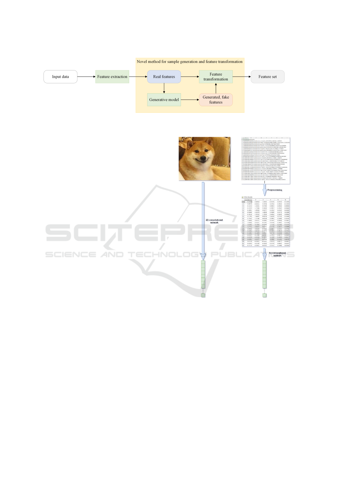
Figure 1: Schematic representation of the model. Adapted to time-series data, it remains the same; only the feature extraction
module had to be changed.
purpose was under construction when the research
was carried out. However, while the database is in-
complete, preliminary tests were conducted using an
available public dataset. In a related endeavor, Jio-
keng et al. devised a distinct biometric authentica-
tion system, which relies on classifying the subject’s
heart signal, detected through the vibrations in their
hand while holding a mobile phone. Their study en-
compassed 112 users, but it posed unique challenges
due to the meaningful signal’s relatively faint and in-
tricate nature. Substantial preprocessing efforts were
required to filter out extraneous information. Impres-
sively, the authors’ model achieved a commendable
level of accuracy. Notably, their experiments were
conducted within a closed-set scenario, wherein the
model’s task was to identify and grant access only to
registered users it had been trained on (Jiokeng et al.,
2022). In contrast, the novel model exhibits the ca-
pacity to maintain high-performance levels within a
closed-set scenario and discern and reject users whose
data it has not encountered during training, thereby
addressing open-set recognition challenges with con-
siderable accuracy. This attribute enhances the secu-
rity and adaptability of the biometric authentication
system the authors are working on, marking a signifi-
cant advancement in this domain.
3 ADAPTING THE MODEL FOR
TIME-SERIES
The model’s first part aims to extract appropriate fea-
tures capable of training the generative model. The
second part of the model classifies these features.
This means that neither the generative part nor the
second part of the model depends on the input data
type; the only concern is to get the features.
The preprocessing broadly followed the method
described in (Jiokeng et al., 2022). The sensors’ mea-
surements were in a single file for each measurement
session. First, the data from the accelerometer and
gyroscope sensors were extracted. The measurements
Figure 2: Comparison of the feature extraction part of the
model in case of image and time-series data. Due to the
different nature of the inputs, different processing methods
were needed, but at the end of the part, both were converted
into a feature vector of the same size. Thus, the rest of the
model works the same way.
were, of course, made on different timestamps by the
two sensors. Moreover, the sampling of the individual
sensors could have been more perfectly uniform, too.
A single time series with six channels was gained by
resampling the data to a fixed sampling frequency, as
both sensors measure along three axes. A bandpass
filter was applied to isolate the relevant frequencies.
The data were also sliced into shorter parts with some
overlap, thus resulting in plenty of training samples.
Once the data is preprocessed, appropriate fea-
tures need to be extracted. Similar to the case of
DMMLACS 2023 - 3rd International Special Session on Data Mining and Machine Learning Applications for Cyber Security
598

Figure 3: The structure of the convolutional network re-
sponsible for feature extraction.
images, the primary approach was using neural net-
works. Convolutional networks work very well on
images that have two spatial dimensions. As time se-
ries has only one dimension (not counting multiple
channels, which are also present in colored images),
it is self-explanatory to use convolutional layers with
1D convolutional layers. The one shown in Figure 3
proved to be the best performing of the several struc-
tures that have been tried. It consists of five blocks
with a doubling number of channels in each block.
The blocks are built of some one-dimensional con-
volutional layers with ReLU activation function, fol-
lowed by a max pooling layer. The structure closely
resembles VGG networks (Simonyan and Zisserman,
2014). The output of the network is a feature vector
with the same size as it was with image datasets. This
is in the spirit of the modular nature of the model, as
it is illustrated in Figure 2.
4 EXPERIMENTAL RESULTS
The model has been comprehensively evaluated by
using the dataset, the details of which are expounded
upon in Section 2.4. It is important to note that to
the best of our knowledge, there is no existing Open-
Set Recognition (OSR) solution specifically tailored
for this dataset. Consequently, our evaluation primar-
ily focuses on closed-set accuracy, drawing a com-
parison with the work presented by (Jiokeng et al.,
2022) as a baseline reference. The first component
of the model, namely the feature extraction module,
is meticulously designed and illustrated in Figure 3.
While adapting the model for the new dataset, the
generative model and the classifier network were re-
tained without any alterations, adhering to the archi-
tecture initially described in our prior work, (Hal
´
asz
et al., 2023). This decision ensures the preservation
of the model’s proven effectiveness and performance
while making necessary adjustments for the new data
domain. The relevant hardware specifications were as
follows.
• Intel(R) Core(TM) i7-9800X CPU @ 3.80 GHz;
• NVIDIA(R) GeForce RTX(TM) 2080 Ti;
• 128 GB RAM.
4.1 Evaluation Metrics
According to a thorough survey on OSR methods
by Geng et al., the most common metrics for eval-
uating open-set performance are AUC and F1 mea-
sure (Geng et al., 2018). In terms of overall accu-
racy or F1 measure, the metric is highly sensitive to
its calibration, in addition to the real effectiveness of a
model. Hence, open-set recognition performance was
evaluated with the two metrics described below.
AUC: The receiver operating characteristic (ROC)
curve is obtained by plotting the true positive rate
(sensitivity) against the false positive rating (1–
specificity) at every relevant threshold setting. The
area under this curve gives a calibration-free mea-
sure of the open-set detection performance (Fawcett,
2006).
Closed Set Accuracy: It is essential that the
model, while being able to reject unknown sam-
ples, retains its closed-set performance. Therefore,
the closed-set accuracy on the test samples of known
classes was also measured.
4.2 Results
The tests were run with different numbers of known
classes, from 10 to 60, increasing by 10 a time.
Each setup was run five times, with different random
known classes each time. To the authors best knowl-
edge, there were no results published of OSR solu-
tion on this database; only the closed-set accuracy by
(Jiokeng et al., 2022) can be observed. With differ-
ent classifiers, this accuracy ranged between 98.27%
and over 99%. Our results are shown in Table 1. In
Adapting Open-Set Recognition Method to Various Time-Series Data
599

Table 1: Closed-set accuracy and Open-set detection AUC performance of the model on time-series data trained on a different
number of classes. With all number of known classes, the measurements were run five times, and the results were averaged.
Also, the standard deviation of the results is presented.
Known classes 10 20 30 40 50 60
Accuracy 0.954 0.940 0.889 0.933 0.915 0.902
STD 0.029 0.025 0.030 0.028 0.023 0.029
AUC 0.700 0.727 0.782 0.770 0.800 0.803
STD 0.046 0.085 0.032 0.062 0.031 0.040
terms of closed-set accuracy, the result fell behind the
closed-set approaches, but it is still high. Besides that,
the model could reject most of the unknown samples.
Moreover, its performance even increases with more
classes it was trained on. The deviation of the results
is very low, indicating the robustness of the model to
the choice of known classes.
A significant advantage of the model over other
generative approaches is that it almost completely
eliminates the cost of generating and using fake sam-
ples while benefiting from the performance gain in
terms of accuracy. This is achieved by generating the
samples in a hidden layer of a much simpler structure,
which needs a much smaller generative model struc-
ture to create appropriate samples, and the fact that
the generated samples do not have to be run through
the first part of the model, which is the more heavy-
weight part with convolutional layers. Measurements
show that this gain in time complexity still holds. The
average runtime of a training epoch of the generative
model on one batch is 5.2ms. This is very close to the
case of training on image datasets, which is unsurpris-
ing considering that the real inputs are features of the
same size. The runtime of a generative model creat-
ing samples in the input space cannot be shown this
time, as there were no published GAN structures spe-
cialized for time-series data. The runtime of the first
part of the model on a batch is 2.1ms, on the second
part 0.23ms. Since the generated samples have to be
run only through the second part of the model, 91%
of runtime required to run the generated samples on
the model can be saved.
5 CONCLUSIONS
In conclusion, our exploration into Open-Set Recog-
nition (OSR) within the context of time-series data
brings forth several critical insights and implications.
OSR represents an invaluable extension of traditional
classification methods, and its paramount relevance
becomes abundantly clear when applied to real-life
scenarios, particularly in the authentication domain,
which is our research’s primary objective.
The very essence of authentication demands a sys-
tem that recognizes known users and effectively dis-
cerns unknown or unauthorized individuals. This is
precisely where OSR steps in, acting as a vital shield
against potential security breaches and unauthorized
access. Our findings underscore the profound impor-
tance of OSR in enhancing the robustness and relia-
bility of authentication systems, reinforcing the need
for its widespread adoption in practical applications.
Furthermore, our research highlights a notable gap
in the existing literature: the need for OSR methods
tailored to time-series data. Our preliminary results
demonstrate promising feasibility in adapting OSR
techniques to time-series datasets, so we anticipate a
burgeoning interest in this field. The fusion of OSR
and time-series data analysis augments the security
and reliability of authentication systems and opens
doors to new possibilities in various other domains
where recognizing unknown patterns within sequen-
tial data is paramount.
There is still room for improvement regarding the
feature extraction. Different neural network models
and utterly different feature mining approaches can
be considered. (Tornai and Scheirer, 2019), (Jiokeng
et al., 2022) show that using statistical features with-
out training can also be efficient. Another possible
approach is to take the Fourier transform of the signal
and use the data in the frequency domain as an input
for various neural network structures. Future work in-
cludes exploring these approaches as well as finding
the best-performing combination of them.
ACKNOWLEDGEMENT
This research was supported by the National Re-
search, Development, and Innovation Office through
the grant TKP2021-NVA-26.
REFERENCES
Bodesheim, P., Freytag, A., Rodner, E., and Denzler, J.
(2015). Local novelty detection in multi-class recog-
DMMLACS 2023 - 3rd International Special Session on Data Mining and Machine Learning Applications for Cyber Security
600

nition problems. In 2015 IEEE Winter Conference on
Applications of Computer Vision, pages 813–820.
Fawcett, T. (2006). An introduction to roc analysis. Pattern
Recognition Letters, 27(8):861–874. ROC Analysis in
Pattern Recognition.
Fumera, G. and Roli, F. (2002). Support vector machines
with embedded reject option. Lecture Notes in Com-
puter Science.
Geng, C., Huang, S.-j., and Chen, S. (2018). Recent ad-
vances in open set recognition: A survey.
Goodfellow, I. J., Pouget-Abadie, J., Mirza, M., Xu, B.,
Warde-Farley, D., Ozair, S., Courville, A., and Ben-
gio, Y. (2014). Generative adversarial nets. In
Proceedings of the 27th International Conference on
Neural Information Processing Systems - Volume 2,
NIPS’14, page 2672–2680, Cambridge, MA, USA.
MIT Press.
Grandvalet, Y., Rakotomamonjy, A., Keshet, J., and Canu,
S. (2008). Support vector machines with a reject op-
tion. volume 21, pages 537–544.
Hal
´
asz, A. P., Al Hemeary, N., Daubner, L. S., Zsedrovits,
T., and Tornai, K. (2023). Improving the perfor-
mance of open-set recognition with generated fake
data. Electronics, 12(6).
Jain, L. P., Scheirer, W. J., and Boult, T. E. (2014). Multi-
class open set recognition using probability of inclu-
sion. In ECCV.
Jiokeng, K., Jakllari, G., and Beylot, A.-L. (2022). I want to
know your hand: Authentication on commodity mo-
bile phones based on your hand’s vibrations. Proc.
ACM Interact. Mob. Wearable Ubiquitous Technol.,
6(2).
J
´
unior, P., Souza, R., Werneck, R., Stein, B., Pazinato, D.,
Almeida, W., Penatti, O., Torres, R., and Rocha, A.
(2017). Nearest neighbors distance ratio open-set clas-
sifier. Machine Learning, 106:1–28.
J
´
unior, P., Wainer, J., and Rocha, A. (2016). Specialized
support vector machines for open-set recognition.
Miller, D., Sunderhauf, N., Milford, M., and Dayoub,
F. (2021). Class anchor clustering: A loss for
distance-based open set recognition. In Proceedings
of the IEEE/CVF Winter Conference on Applications
of Computer Vision (WACV), pages 3570–3578.
Rudd, E. M., Jain, L. P., Scheirer, W. J., and Boult, T. E.
(2018). The extreme value machine. IEEE Transac-
tions on Pattern Analysis and Machine Intelligence,
40:762–768.
Scheirer, W. J., Rocha, A., Sapkota, A., and Boult, T. E.
(2013). Toward open set recognition. IEEE Trans-
actions on Pattern Analysis and Machine Intelligence,
35:1757–1772.
Simonyan, K. and Zisserman, A. (2014). Very Deep Con-
volutional Networks for Large-Scale Image Recogni-
tion. arXiv e-prints, page arXiv:1409.1556.
Tornai, K. and Scheirer, W. J. (2019). Gesture-based user
identity verification as an open set problem for smart-
phones. In IAPR International Conference On Bio-
metrics.
Wan, L., Zeiler, M., Zhang, S., Cun, Y. L., and Fergus, R.
(2013). Regularization of neural networks using drop-
connect. In Dasgupta, S. and McAllester, D., editors,
Proceedings of the 30th International Conference on
Machine Learning, volume 28 of Proceedings of Ma-
chine Learning Research, pages 1058–1066, Atlanta,
Georgia, USA. PMLR.
Adapting Open-Set Recognition Method to Various Time-Series Data
601