A Comparison Between Seasonal and Non-Seasonal Forecasting
Techniques for Energy Demand Time Series in Smart Grids
Sabereh Taghdisi Rastkar, Danial Zendehdel, Enrico De Santis
a
and Antonello Rizzi
b
Department of Information Engineering, Electronics and Telecommunications,
Sapienza University of Rome, 00185 Roma, Italy
Keywords:
Time Series Energy Forecasting, Forecasting Algorithm, Seasonality Effect.
Abstract:
Accurate energy consumption forecasting is essential for optimizing resource allocation and ensuring a reliable
energy supply. This paper conducts a thorough analysis of energy consumption forecasting using XGBoost,
SARIMA, LSTM, and Seasonal-LSTM algorithms. It utilizes two years of hourly electricity demand data
from Italy and the PJM region (USA), categorizing algorithms into seasonality and non-seasonality groups.
Performance metrics like RMSE, MAE, R
2
, and MSPE are employed. The study underscores the importance
of considering seasonality, with SARIMA and Seasonal-LSTM achieving high accuracy in the seasonality
group. In the non-seasonality group, XGBoost and LSTM perform competitively. In summary, this research
aids in choosing suitable forecasting algorithms for building an Energy Management System for smart energy
management in microgrids, considering seasonality and data attributes. These insights can also benefit energy
companies in efficient resource management, promoting sustainable energy practices and urban development.
1 INTRODUCTION
Consider an urban area that relies solely on renewable
energy sources. In this setting, accurately predicting
energy consumption and demand during different sea-
sons and public holidays becomes critical. However,
forecasting the utility consumption aids in balancing
the generation and demand of energy.
Energy consumption problems have become a
practical research topic in recent years. Energy prob-
lems are crucial for the security and well-being of so-
cieties (Ghalehkhondabi et al., 2017). However, un-
like many other energy sources, electricity must be
consumed immediately after generation. Thus, fore-
casting future electricity demand is vital for power
companies to allocate resources and guarantee suf-
ficient supply effectively. This information about
consumption and demand aids firms in implementing
unique energy conservation strategies, as storing elec-
tricity is often prohibitively expensive, inefficient, or
unfeasible. Consequently, balancing electricity con-
sumption and generation becomes critical (Nguyen
and Hansen, 2017). Thus, forecasting future power
demand is crucial for power companies in their en-
a
https://orcid.org/0000-0003-4915-0723
b
https://orcid.org/0000-0001-8244-0015
ergy management efforts (Hamzac¸ebi et al., 2019).
Moreover, the growing world population and increas-
ing use of advanced technologies are expected to drive
electricity demand. The emergence of smart grids
has made load prediction systems indispensable for
sustainable growth and intelligent urban development
(Azeem et al., 2021). With the advent of intelligent
networks, power demand forecasting will become in-
creasingly important (Hamzac¸ebi et al., 2019).
Moreover, Renewable Energy Communities
equipped with Intelligent Energy Management
Systems (EMS) have emerged as potent catalysts
for change. These communities, which leverage
a combination of renewable energy sources like
solar, wind, and hydro, are reshaping production and
consumption. However, the variable and stochastic
nature of renewable energy generation presents
unique challenges that require sophisticated man-
agement strategies. Hence, a high-performance
forecasting system plays a significant role in tackling
this problem. Accurate and reliable energy consump-
tion and production forecasts are the backbone of
any effective EMS. A well-calibrated forecasting
model can enable real-time adjustments to energy
distribution, ensuring supply reliably meets demand
while minimizing waste. In this way, advanced
Rastkar, S., Zendehdel, D., De Santis, E. and Rizzi, A.
A Comparison Between Seasonal and Non-Seasonal Forecasting Techniques for Energy Demand Time Series in Smart Grids.
DOI: 10.5220/0012265900003595
In Proceedings of the 15th International Joint Conference on Computational Intelligence (IJCCI 2023), pages 459-467
ISBN: 978-989-758-674-3; ISSN: 2184-3236
Copyright © 2023 by SCITEPRESS – Science and Technology Publications, Lda. Under CC license (CC BY-NC-ND 4.0)
459

forecasting is not merely an adjunct but a central
component of an Intelligent EMS in enhancing both
Renewable Energy Communities’ economic and
environmental sustainability.
Load forecasting has been a long-standing tech-
nique used to predict future demand. It plays a
critical role in the precise design and placement of
electrical loads at various time intervals within the
planning horizon. Therefore, the potentially signifi-
cant cost savings of accurate load forecasts bring sig-
nificant benefits to electrical utilities (Singh et al.,
2012). Predicting load demand and managing elec-
tricity are essential for energy conservation (Nepal
et al., 2020). Numerous forecasting algorithms have
been devised to enhance forecast accuracy, each with
unique strengths and weaknesses. Selecting the ideal
algorithm for a given situation requires comparing
various algorithms in different settings. Understand-
ing data trends and their association with different
types of seasonality is crucial for accurately predict-
ing energy demand (Hong et al., 2016). For instance,
air conditioning increases during warm months, lead-
ing to higher power consumption. Conversely, the de-
mand for heating rises in colder seasons, affecting en-
ergy usage. Energy consumption also fluctuates on
holidays and weekends.
In this study, we categorize forecasting techniques
into two primary groups: those reliant on season-
ality, such as SARIMA and seasonality LSTM, and
those independent of it, represented by XGBoost and
LSTM. We will then conduct a comprehensive analy-
sis of these methods and their inherent characteristics.
This inquiry underscores the significance of utilizing
precise forecasting techniques and tools to ensure a
dependable energy supply and enhance energy man-
agement. Lastly, we will assess the performance of
these methods on diverse data sets using metrics such
as mean absolute error, mean square percentage error,
and root mean square error.
The remainder of this study is organized as fol-
lows. In Sec. 2 the technical literature is revised. In
Sec. 3
2 RELATED WORK
The growing importance of energy forecasting in the
business sector is undeniable, particularly in the field
of renewable energies. Accurate demand forecasting
is vital for energy planning, efficient resource allo-
cation, and cost savings for energy suppliers. Over
the years, traditional forecasting techniques have been
developed to predict energy demand and have histori-
cally been reliable. However, the increasing complex-
ity of the energy system and the advent of new tech-
nologies may render these traditional methods insuf-
ficient. These traditional mathematical models, based
on the Box and Jenkins method, are mainly statisti-
cal and they are categorized as linear methods that
employ a linear functional form for the time-series
models. It encloses the Auto-Regressive Integrated
Moving-Average (ARIMA) model (Wang et al., 2012;
Yukseltan et al., 2017; Amini et al., 2016; Debuss-
chere et al., 2012), exponential smoothing model
(Chen et al., 2010), linear model (Zhou, 2017), and re-
gression analysis methods (Fumo and Biswas, 2015;
Amber et al., 2015).
Moreover, some mature nonlinear methods, such
as Artificial Neural Networks (ANNs) (Tian and Hao,
2018; Ganesan et al., 2015) and Support Vector Ma-
chines (SVMs) (Zhang and Wang, 2018), have been
employed. For instance, some studies showed that
a range of energy demand forecasting models for
time series, such as regression and soft computing
techniques (including fuzzy logic, genetic algorithms,
neural networks, and support vector regression), are
extensively used for demand side management (Singh
et al., 2012; Avami and Boroushaki, 2011; Suganthi
and Samuel, 2012). The ANNs are limited by insuf-
ficient data for accurate forecasting (Tian and Hao,
2018). Neural networks need many control parame-
ters, which have difficulties getting a stable solution,
risks of over-fitting, and restraint by insufficient data
(Tian and Hao, 2018; Ganesan et al., 2015). Along-
side machine-learning algorithms, Deb (Deb et al.,
2017) thoroughly reviewed existing machine-learning
techniques and ANNs for forecasting time-series en-
ergy consumption. In 2017, the BRE Trust Centre
reviewed machine-learning algorithms like artificial
neural networks, support vector machines, and time
series analysis for short and very short-term predic-
tion, evaluating their performance using several met-
rics (Kuster et al., 2017). More recently, a study ex-
amined eight methods for predicting electricity de-
mand in supermarkets, schools, and residential build-
ings at the individual structure level, employing statis-
tics, machine learning, and a median ensemble tech-
nique (Groß et al., 2021). Additionally, researchers
at the University of Brasilia utilized regularized ma-
chine learning models to predict short- and medium-
term energy consumption in Brazil, comparing them
against standard criteria such as the Random Walk
and the ARIMA(Albuquerque et al., 2022).
Seasonality is a characteristic of a time series in
which the data experiences regular and predictable
changes that recur every calendar year. These changes
are often influenced by the seasons of the year,
holidays, and other recurring events. Seasonality
NCTA 2023 - 15th International Conference on Neural Computation Theory and Applications
460

can significantly impact the patterns and trends ob-
served in time-series data. In 2008, Lam consid-
ered the effect of seasonal variations on used en-
ergy, mainly caused by air-conditioning requirements
changes (Lam et al., 2008). Additionally, holiday pe-
riods can cause spikes in energy consumption due to
increased activities in homes and commercial estab-
lishments. A study by the U.S. Energy Information
Administration highlighted the significant seasonal
variation in energy consumption across the country,
attributing it to weather-related factors, holiday pat-
terns, and even the academic calendar (Outlook et al.,
2010). Furthermore, the length of the day can also
play a role, with longer daylight hours in the summer
leading to reduced lighting needs.
Several researchers have also explored method-
ologies to address seasonality in energy consumption
forecasting. In a study by Rashedul, the seasonal de-
composition of time series (STL) approach was pro-
posed to model and predict energy consumption, ef-
fectively capturing the seasonality patterns (Haq and
Ni, 2019). In another study, Xiong significantly im-
proved the accuracy and speed of forecasting energy
consumption (Xiong et al., 2021). Moreover, sev-
eral studies focused on seasonal SARIMA. For in-
stance, Wang presented a combination of PSO opti-
mal Fourier method models with seasonal ARIMA for
energy consumption prediction (Wang et al., 2012).
This research aims to compare traditional and ad-
vanced techniques for electrical load forecasting to
assist suppliers in selecting efficient methods, consid-
ering impact of seasonality, and ensuring long-term
sustainability.
3 METHODOLOGY
The methodology outlined in this study involves sev-
eral crucial steps designed to compare energy con-
sumption prediction results while accounting for sea-
sonality’s influence. We have categorized our ap-
proach into two groups as follows:
• Group A: Non-seasonal forecasting models
• Group B: Seasonal forecasting models
In each of these groups, A and B, we have included
two distinct forecasting models. Group A comprises
the XGBoost (Wang et al., 2021) (Phan et al., 2021)
and LSTM algorithms, while Group B integrates the
SARIMA and Seasonal-LSTM models. We have ap-
plied these four forecasting algorithms (XGBoost,
SARIMA, Seasonal-LSTM, and LSTM) to the two
distinct datasets previously mentioned - see Sec. 4.1
below. To ensure precise predictions, we have cus-
tomized the models to align with the unique char-
acteristics of each dataset, using Python. The sub-
sequent section will provide a comprehensive break-
down of the methodology employed for forecasting
energy consumption.
3.1 System Model
In this section, we offer a summary of the fundamen-
tal elements and procedures required to create a sys-
tem model that integrates various machine learning
algorithms. Figure 1 presents a holistic perspective of
the steps involved in time series forecasting as con-
ducted in this study.
Figure 1: Flow chart of time series energy forecasting.
3.2 Seasonal Effects
Seasonality in time series data refers to regular and
predictable changes that occur annually, often tied to
seasons, holidays, and recurring events. These pat-
terns significantly influence the observed data trends.
In the context of energy consumption, seasonality is
pronounced due to factors like weather variations,
leading to increased heating or cooling needs during
extreme seasons. Holidays can also cause spikes in
energy use, as can the length of daylight hours. Ne-
glecting seasonality in energy consumption forecast-
ing models can lead to inaccurate predictions. Exist-
ing research highlights that accounting for seasonal-
ity greatly improves forecasting model accuracy, ulti-
mately aiding in more effective energy planning and
management.
3.3 Algorithm Description
This section provides concise explanations of each
forecasting algorithm utilized in this study.
Non-seasonal forecasting models:
• LSTM (Long Short-Term Memory), a type of re-
current neural network (RNN), is well-suited for
A Comparison Between Seasonal and Non-Seasonal Forecasting Techniques for Energy Demand Time Series in Smart Grids
461

sequence prediction tasks, particularly in time se-
ries forecasting. This study configures the LSTM
model with three LSTM layers, each containing
40 units. Dropout layers with a 0.2 dropout rate
are incorporated to prevent overfitting. The model
processes sequences of length 20, effectively cap-
turing temporal dependencies to make single pre-
dictions. With 32,681 trainable parameters, the
model is designed to decode complex time series
trends, enhancing its capability to uncover intri-
cate data patterns.”
• XGBoost (Extreme Gradient Boosting) is a pow-
erful machine learning algorithm for accurate
forecasting by combining predictions from mul-
tiple decision trees. It’s known for its efficiency
and versatility, suitable for various forecasting
tasks. The model in use is configured as a re-
gression model, with extensive hyperparameters,
100,000 boosting rounds, a learning rate of 0.05,
max depth of 5, no gamma value, 80% subsam-
pling, and objective function ’reg:squarederror’.
Seasonal forecasting models:
• SARIMA (Seasonal Autoregressive Integrated
Moving Average) enhances upon ARIMA for sea-
sonal time series data, introducing three seasonal
parameters (P, D, Q) and a seasonality factor ’s.’
The provided SARIMA model is adaptable to var-
ious data sets. Auto ARIMA from pmdarima au-
tomatically tunes model parameters. SARIMA or-
der is extracted, and SARIMAX is initialized for
training. A rolling forecast predicts test data, re-
peatedly re-optimizing SARIMA.
• Seasonality decomposition in LSTM forecasting
entails the dissection of a time series into its con-
stituent parts: seasonal, trend, and residual com-
ponents. This dissection is critical for gaining
a deeper comprehension of the time series’ pat-
terns and fluctuations, thereby enabling more ac-
curate predictions. By separating these compo-
nents, LSTM models can adeptly harness sea-
sonality information, significantly enhancing their
forecasting capabilities. To execute this decompo-
sition of time series data, the seasonal decompo-
sition method from the statsmodels library is em-
ployed.
4 EXPERIMENTAL RESULT
4.1 Data Sets
This research utilizes four distinct data sets sourced
by Kaggle. Each data set offers unique insights into
different energy consumption scenarios, providing a
broad spectrum of data for the analysis. All data sets
comprise two columns: the observation date and the
corresponding energy consumption value. The date
column captures the chronological progression of the
data, while the energy consumption column measures
the actual energy usage. These data sets were specif-
ically selected for their relevance and potential to re-
veal valuable patterns and trends influencing energy
consumption. In our training, we modified the en-
ergy consumption data from an hourly to a 6-hourly
frequency. This change is because the original data
set exhibited strong seasonality, leading to high com-
plexity in the models. By aggregating the data into 6-
hour intervals, we effectively reduced the complexity
and produced a more condensed time series, allowing
the models to fetch the underlying patterns and trends.
We provide a detailed description of each data set. We
focused on hourly data from the past two years of the
following data sets:
• PJM Hourly Energy Demand for the years 2016-
2018
1
(Albuquerque et al., 2022) (Khan et al.,
2022).
• Italy’s Hourly Energy Consumption for 2020-
2022
2
(Lisi and Edoli, 2018)(Rossi and Brunelli,
2013).
Furthermore, Figure 2 provides a clear presen-
tation of the mean features extracted from the two
data sets illustrated in Figure A (PJM) and Figure
B (Italy). These features are derived using the XG-
Boost algorithm, which employs an iterative process
of constructing decision trees and assessing the im-
pact of each feature on the model’s predictive accu-
racy. This information holds significant value, as it
aids in discerning the most pertinent and influential
features within the data set (feature selection).
4.2 Evaluation Metrics
Common metrics used to evaluate forecast accuracy
include Mean Absolute Error (MAP) and other evalu-
ation metrics such as RMSE and MSPE, in addition to
them we have used R-Squared (R
2
) as a measure that
compares the stationary part of the model to a simple
mean model. R
2
can be evaluated by 1. This metric,
also known as the coefficient of determination, mea-
sures the proportion of the variance in the actual ob-
1
https://www.kaggle.com/datasets/robikscube/
hourly-energy-consumption
2
https://www.kaggle.com/datasets/paolodelia/
italian-electric-market-data
NCTA 2023 - 15th International Conference on Neural Computation Theory and Applications
462

(a) feature important in PJM data set .
(b) feature important in Italy data set.
Figure 2: Feature important in PJM and Italy data sets .
servations that is explained by the predicted values.
R
2
= 1 −
SS
res
SS
tot
(1)
In Eq. 1 SS
res
is the Sum of the Square of Resid-
uals. Here, residual is the difference between pre-
dicted and actual values, and SS
tot
is the Total Sum
of Squares.
4.3 Simulation Result
In this section, we conduct rigorous experiments
on two sets of forecasting algorithms (XGBoost,
SARIMA, LSTM, Seasonal-LSTM) using two years
of hourly electricity demand data. Our main objective
is to evaluate each model’s forecasting accuracy. The
focus is on comparing algorithm outcomes concern-
ing seasonality considerations.
Figure3 visually illustrates the energy consump-
tion patterns in Italy and the United States throughout
the week, emphasizing a significant rise during week-
days and a subsequent decline as the week progresses
toward the weekend. It is notable that the highest en-
ergy consumption occurs at the end of each weekday.
Figure 4 shows seasonality decomposition of PJM
data set of energy consumption visualized in separate
figures of trend,seasonality and residual.
(a) Weekly graph of energy demand in Italy.
(b) Weekly graph of energy demand in PJM data set.
Figure 3: Weekly graphs of energy demand in PJM and Italy
data sets.
Figure 4: Seasonal decomposition of PJM energy consump-
tion data set.
Within the category of seasonality forecasting
models, Figure 5a illustrates the prediction results of
the SARIMA model, configured with non-seasonal
orders of (1, 0, 4) and seasonal orders of (4, 1, [1,
2], 12), applied to the PJM data set. Conversely,
Figure 5b showcases the prediction outcomes of the
SARIMA model, specifically configured as SARI-
MAX(3, 0, 4)x(4, 1, [1, 2], 12) in Italy data set.
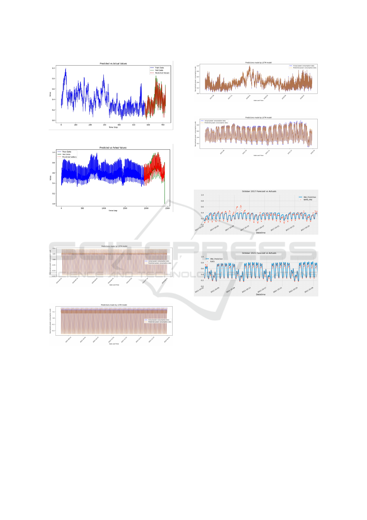
Figure 6 depicts a comparison of the actual and
predicted energy consumption in both PJM and Italy
data sets, respectively. This comparison is based on
the results generated by the seasonal LSTM forecast-
ing algorithm.The graph provides a visual representa-
tion of how closely the predicted values align with the
real data.
In the group without seasonality considerations,
Figure 7 displays the results of the LSTM algorithm’s
energy consumption forecasting. This figure offers
a visual comparison between the actual energy con-
sumption and the model’s predictions. The X-axis
represents time, while the Y-axis represents energy
consumption levels. This visual assessment allows us
to gauge the accuracy and performance of the predic-
tion model. Any disparities between the actual and
predicted values may indicate areas where further im-
provements to the model are needed.
A Comparison Between Seasonal and Non-Seasonal Forecasting Techniques for Energy Demand Time Series in Smart Grids
463

(a) Result of SARIMA model forecasting energy de-
mand in PJM data set.
(b) Result of SARIMA model forecasting energy de-
mand in Italy data set.
Figure 5: Graph of Train, test and predicted Result of
SARIMA model in PJM and Italy data sets.
(a) plot of the LSTM model with seasonal decomposition
in PJM data set.
(b) plot of the LSTM model with seasonal decomposi-
tion in Italy data set.
Figure 6: Predicted and actual energy consumption plot of
the LSTM model with seasonal decomposition in PJM and
Italy data sets.
The final algorithm in the non-seasonal group is
XGBoost. Figure 8 illustrates the energy consump-
tion forecasting results generated by this model for
two specific dates within a one-month period. The
figure demonstrates that the forecasting model has
achieved a reasonably successful alignment with the
actual energy consumption patterns.
Table 1 showcases the outcomes of both seasonal
(a) Model train and validation loss of the LSTM model,
PJM data set.
(b) Model train and validation loss of the LSTM model,
Italy data set.
Figure 7: Model train and validation loss of the LSTM
model in PJM and Italy data sets.
(a) Model train and validation loss of the XGBoost
model in October 2017, PJM data set.
(b) Model train and validation loss of the XGBoost
model in October 2021, Italy data set.
Figure 8: Forecasting energy demand in PJM and Italy data
sets with XGBoost algorithm.
and non-seasonal models, enabling a comparison of
how seasonality impacts time series forecasting.
5 CONCLUSIONS
This study has provided valuable insights into the
realm of energy consumption forecasting, a critical
component for optimizing resource allocation and en-
suring a dependable energy supply. We conducted
a rigorous evaluation of four distinct forecasting al-
gorithms, namely XGBoost, SARIMA, LSTM, and
Seasonal-LSTM, utilizing two years’ worth of hourly
electricity demand data from both Italy and the PJM
region.
Our findings underscore the paramount impor-
NCTA 2023 - 15th International Conference on Neural Computation Theory and Applications
464

Table 1: Result of two forecasting models groups for PJM and Italy data sets.
ITALY PJM
RMSE MAE R
2
MSPE RMSE MAE R
2
MSPE
seasonality
SARIMA 0.0492 0.0302 0.889 0.4933 0.0567 0.0423 0.9155 6.0194
S-LSTM 0.0087 0.007 0.9965 420.8256 0.0054 0.0043 0.995 3116.8796
Non seasonality
XGBoost 0.0601 0.0424 0.9094 2.6651 0.12 0.0914 0.515 19.7695
LSTM 0.0228 0.0174 0.9869 69.9224 0.0177 0.0134 0.9889 123.554
tance of accounting for seasonality when forecasting
energy consumption. Within the seasonality group,
the SARIMA and Seasonal-LSTM models emerged
as standout performers, exhibiting exceptional accu-
racy with R
2
values that nearly approached 1. These
models adeptly captured the inherent seasonal pat-
terns in energy consumption, showcasing their robust
forecasting capabilities.
In contrast, the non-seasonality group witnessed
competitive performances from the XGBoost and
LSTM models. While their R
2
values were slightly
lower, they still demonstrated strong forecasting
prowess, with LSTM particularly noteworthy for
achieving an impressive R
2
score of 0.98.
The results presented in Table 1 reinforce the su-
periority of seasonality-aware models, with SARIMA
and Seasonal-LSTM outperforming others by achiev-
ing lower RMS E and MSPE values while securing
higher R
2
scores. These models excelled in effec-
tively capturing and leveraging the cyclic variations
in energy consumption.
It’s also worth noting that the performance of each
model varies depending on the data set. For in-
stance, LSTM with seasonal decomposition exhibited
a high value for MSPE in PJM data sets. This high-
lights the importance of data set-specific considera-
tions when comparing the results of SARIMA and
LSTM with seasonal decomposition in the seasonal-
ity model group. SARIMA inherently possesses sea-
sonal properties within the algorithm, while LSTM
with seasonal decomposition incorporates these prop-
erties externally.
Nonetheless, it’s essential to acknowledge that
other factors, such as weather conditions, can signifi-
cantly influence the forecasting outcomes, potentially
impacting algorithm selection for a given time series
data set.
In conclusion, this research serves as a valuable
resource for selecting appropriate forecasting algo-
rithms, considering seasonality and data characteris-
tics. Its insights hold great potential for energy com-
panies seeking to elevate their resource management
practices, thereby contributing to sustainable energy
strategies and intelligent urban development. The
utilization of accurate forecasting models can sub-
stantially enhance the allocation and optimization of
energy resources, establishing them as indispensable
tools in today’s dynamic energy landscape.
ACKNOWLEDGEMENTS
This study was carried out within the MOST –
Sustainable Mobility Center and received funding
from the European Union Next-GenerationEU (PI-
ANO NAZIONALE DI RIPRESA E RESILIENZA
(PNRR) – MISSIONE 4 COMPONENTE 2, IN-
VESTIMENTO 1.4 – D.D. 1033 17/06/2022,
CN00000023). This manuscript reflects only the
authors’ views and opinions, neither the European
Union nor the European Commission can be consid-
ered responsible for them.
REFERENCES
Albuquerque, P. C., Cajueiro, D. O., and Rossi, M. D.
(2022). Machine learning models for forecasting
A Comparison Between Seasonal and Non-Seasonal Forecasting Techniques for Energy Demand Time Series in Smart Grids
465

power electricity consumption using a high dimen-
sional dataset. Expert Systems with Applications,
187:115917.
Amber, K., Aslam, M., and Hussain, S. (2015). Electric-
ity consumption forecasting models for administration
buildings of the uk higher education sector. Energy
and Buildings, 90:127–136.
Amini, M. H., Kargarian, A., and Karabasoglu, O. (2016).
Arima-based decoupled time series forecasting of
electric vehicle charging demand for stochastic power
system operation. Electric Power Systems Research,
140:378–390.
Avami, A. and Boroushaki, M. (2011). Energy consumption
forecasting of iran using recurrent neural networks.
Energy Sources, Part B: Economics, Planning, and
Policy, 6(4):339–347.
Azeem, A., Ismail, I., Jameel, S. M., and Harindran, V. R.
(2021). Electrical load forecasting models for differ-
ent generation modalities: a review. IEEE Access,
9:142239–142263.
Chen, J., Ji, P., and Lu, F. (2010). Exponential smoothing
method and its application to load forecasting. Jour-
nal of China Three Gorges University (Natural Sci-
ence Edition), 32(03):37–4.
Deb, C., Zhang, F., Yang, J., Lee, S. E., and Shah, K. W.
(2017). A review on time series forecasting techniques
for building energy consumption. Renewable and Sus-
tainable Energy Reviews, 74:902–924.
Debusschere, V., Bacha, S., et al. (2012). One week
hourly electricity load forecasting using neuro-fuzzy
and seasonal arima models. IFAC Proceedings Vol-
umes, 45(21):97–102.
Fumo, N. and Biswas, M. R. (2015). Regression analysis
for prediction of residential energy consumption. Re-
newable and sustainable energy reviews, 47:332–343.
Ganesan, P., Rajakarunakaran, S., Thirugnanasambandam,
M., and Devaraj, D. (2015). Artificial neural network
model to predict the diesel electric generator perfor-
mance and exhaust emissions. Energy, 83:115–124.
Ghalehkhondabi, I., Ardjmand, E., Weckman, G. R., and
Young, W. A. (2017). An overview of energy demand
forecasting methods published in 2005–2015. Energy
Systems, 8:411–447.
Groß, A., Lenders, A., Schwenker, F., Braun, D. A., and
Fischer, D. (2021). Comparison of short-term elec-
trical load forecasting methods for different building
types. Energy Informatics, 4:1–16.
Hamzac¸ebi, C., Es, H. A., and C¸ akmak, R. (2019). Fore-
casting of turkey’s monthly electricity demand by sea-
sonal artificial neural network. Neural Computing and
Applications, 31:2217–2231.
Haq, M. R. and Ni, Z. (2019). A new hybrid model for
short-term electricity load forecasting. IEEE access,
7:125413–125423.
Hong, T., Pinson, P., Fan, S., Zareipour, H., Troccoli, A.,
and Hyndman, R. J. (2016). Probabilistic energy fore-
casting: Global energy forecasting competition 2014
and beyond.
Khan, Z. A., Ullah, A., Haq, I. U., Hamdy, M., Mauro,
G. M., Muhammad, K., Hijji, M., and Baik, S. W.
(2022). Efficient short-term electricity load forecast-
ing for effective energy management. Sustainable En-
ergy Technologies and Assessments, 53:102337.
Kuster, C., Rezgui, Y., and Mourshed, M. (2017). Electrical
load forecasting models: A critical systematic review.
Sustainable cities and society, 35:257–270.
Lam, J. C., Tang, H. L., and Li, D. H. (2008). Seasonal vari-
ations in residential and commercial sector electricity
consumption in hong kong. Energy, 33(3):513–523.
Lisi, F. and Edoli, E. (2018). Analyzing and forecasting
zonal imbalance signs in the italian electricity market.
The Energy Journal, 39(5).
Nepal, B., Yamaha, M., Yokoe, A., and Yamaji, T. (2020).
Electricity load forecasting using clustering and arima
model for energy management in buildings. Japan Ar-
chitectural Review, 3(1):62–76.
Nguyen, H. and Hansen, C. K. (2017). Short-term elec-
tricity load forecasting with time series analysis. In
2017 IEEE International Conference on Prognostics
and Health Management (ICPHM), pages 214–221.
IEEE.
Outlook, A. E. et al. (2010). Energy information adminis-
tration. Department of Energy, 92010(9):1–15.
Phan, Q. T., Wu, Y. K., and Phan, Q. D. (2021). A hybrid
wind power forecasting model with xgboost, data pre-
processing considering different nwps. Applied Sci-
ences, 11(3):1100.
Rossi, M. and Brunelli, D. (2013). Electricity demand fore-
casting of single residential units. In 2013 IEEE Work-
shop on Environmental Energy and Structural Moni-
toring Systems, pages 1–6. IEEE.
Singh, A. K., Khatoon, S., Muazzam, M., Chaturvedi,
D., et al. (2012). Load forecasting techniques and
methodologies: A review. In 2012 2nd International
Conference on Power, Control and Embedded Sys-
tems, pages 1–10. IEEE.
Suganthi, L. and Samuel, A. A. (2012). Energy models for
demand forecasting—a review. Renewable and sus-
tainable energy reviews, 16(2):1223–1240.
Tian, C. and Hao, Y. (2018). A novel nonlinear com-
bined forecasting system for short-term load forecast-
ing. Energies, 11(4):712.
Wang, Y., Sun, S., Chen, X., Zeng, X., Kong, Y., Chen,
J., Guo, Y., and Wang, T. (2021). Short-term load
forecasting of industrial customers based on svmd and
xgboost. International Journal of Electrical Power &
Energy Systems, 129:106830.
Wang, Y., Wang, J., Zhao, G., and Dong, Y. (2012). Appli-
cation of residual modification approach in seasonal
arima for electricity demand forecasting: A case study
of china. Energy Policy, 48:284–294.
Xiong, X., Hu, X., and Guo, H. (2021). A hybrid optimized
grey seasonal variation index model improved by
whale optimization algorithm for forecasting the resi-
dential electricity consumption. Energy, 234:121127.
Yukseltan, E., Yucekaya, A., and Bilge, A. H. (2017). Fore-
casting electricity demand for turkey: Modeling peri-
odic variations and demand segregation. Applied En-
ergy, 193:287–296.
NCTA 2023 - 15th International Conference on Neural Computation Theory and Applications
466

Zhang, X. and Wang, J. (2018). A novel decomposition-
ensemble model for forecasting short-term load-time
series with multiple seasonal patterns. Applied Soft
Computing, 65:478–494.
Zhou, G. (2017). Design, Fabrication and Electrochemical
Performance of Nanostructured Carbon Based Mate-
rials for High-Energy Lithium–Sulfur Batteries: Next-
Generation High Performance Lithium–Sulfur Batter-
ies. Springer.
A Comparison Between Seasonal and Non-Seasonal Forecasting Techniques for Energy Demand Time Series in Smart Grids
467