Research on Color Vision Tool Design Based on Detection Algorithms

Kun Zhang, Bo Zhang, Yue-wu Li, Shao-guang Zhang, Yu-sen Tao and Yong-xu Liu

The Army Engineering University of PLA, Nanjing, China

Keywords: Detection Algorithm, Color Vision Tool, Target Recognition.

Abstract: Accurate identification can quickly determine the state of the target, which is of great significance in both

military and industrial production. This article designs several sets of experiments based on detection algo-

rithms to evaluate the applicability and operational efficiency of color detection tools. The experimental re-

sults show that, compared with the color detection tool in Cognex DIP, the color detection tool basically

meets the design requirements and is equivalent in efficiency to the reference software. It can be applied to

military target recognition and industrial applications.

1 INTRODUCTION

In the field of military applications, accurately

identifying targets can improve rapid response

capabilities, and accurately identifying unexploded

ordnance can provide accurate positioning.

Therefore, rapid recognition technology has broad

application space and significant practical

significance in the future. The design of color visual

tools mainly includes two aspects: firstly, color

feature extraction; The second is the measurement of

color difference. In the conventional design field, the

hue component (H component) in the color space

based on human visual characteristics represents the

fundamental color, i.e. the main wavelength of the

spectrum. The distribution of the hue histogram

represents the overall color distribution of the target

(Ma Rui-qing, 2019). When identifying non

functional targets or the product coloring is incorrect,

it will be reflected on the hue histogram. Therefore,

by comparing the difference in hue histograms

between the current target image and the template

image, it is determined whether the current product

coloring is correct (or acceptable), and then the

target is identified and distinguished.

2 DESIGN REQUIREMENTS

The design requirements for color visual tools

mainly include the following aspects: 1) Color

feature selection: Provide at least one color feature

for color detection. 2) Color difference measurement:

provide at least one color difference measurement

method. 3) Applicability: It can be applied to several

application scenarios, such as identifying military

targets or inspecting the coloring degree of industrial

products. 4) Job efficiency: It is equivalent to the

reference software in terms of work time scale, at

the same level of magnitude. According to the

design principles and requirements, develop a basic

algorithm for color detection, as shown in Figure 1

(

Safdar, 2017).

Figure 1: Basic framework diagram of color detection

algorithm.

Zhang, K., Zhang, B., Li, Y., Zhang, S., Tao, Y. and Liu, Y.

Research on Color Vision Tool Design Based on Detection Algorithms.

DOI: 10.5220/0012273100003807

Paper published under CC license (CC BY-NC-ND 4.0)

In Proceedings of the 2nd International Seminar on Artiﬁcial Intelligence, Networking and Information Technology (ANIT 2023), pages 20-25

ISBN: 978-989-758-677-4

3 COLOR FEATURE

EXTRACTION

Color features mainly refer to the description of the

color information of an image (or product), such as

how much red it contains and how much blue it

contains. Although the RGB color space also

contains color information, it is difficult to quantify

and the expression is not intuitive enough. The hue

components in HSI color space intuitively describe

basic color information. The statistical histogram

distribution based on hue components represents the

overall color distribution of the product, therefore,

hue histograms can be used as color features for

color detection.

3.1 HSI Color Space

Figure 2: HSI color space.

The HSI color space separates the intensity of colors

from color information, which is determined by light

intensity, while color information is described by

two parameters: hue and saturation. Hue represents

the basic color, which is the main wavelength of the

spectrum. Saturation is a measure of the purity of a

color, representing the amount of mixed white light

in the color, which is the ratio of peak height to the

entire spectral distribution. The geometric

description of the HSI color space is shown in

Figure 2, which is a cylindrical coordinate space

(Shamey, 2015). The color tone in the figure is

described as the angle between the ray formed by the

center of the cylinder and the color point to the

reference line, with a range of 0°~360°; Saturation is

described as the ray distance from the color point to

the center of the cylinder; Brightness is expressed as

the axial height, and the plane perpendicular to the

brightness axis in a cylinder is a first order

brightness plane. The mapping relationship between

HSI color space and RGB color space is:







>−

≤

GBif

,360





















−−+−

−+−

−

2/12

)])(()[(

)]()[(

cos

BGBRGR

BRGR

(1)

{}

BGR

S ,,min

)(

−=

;

(2)

3/)( BGRI ++=

(3)

For the convenience of processing, the range of

values for the H, S, and I components is uniformly

adjusted to [0,255].

3.2 Tone Histogram and Filtering

Processing

The hue histogram of an image is a one-dimensional

discrete function

ℎ(𝑘)=𝑛



, 𝑘 =0,1,⋯ ,255

(4)

Among them,ℎ(𝑘) is the image hue histogram, n

the sum of the hue values in the image equal to the

number of k pixels, and the hue value range of the

image is [0,255].

(a) Input RGB image

(b) Color tone histogram of input RGB

Figure 3: Hue histogram.

Figure 3 shows a schematic diagram of an image

tone histogram. The rectangular area of the image

shown in Figure 3 (a) mainly contains two tones,

one is blue as the background and the other is green

as the target. Figure 3 (b) is a hue histogram of the

rectangular area of the image in Figure 3 (a). It can

be seen from the graph that the two peaks in the hue

histogram correspond exactly to blue and green.

Therefore, tone histograms can effectively reflect the

content of a certain color in an image.

According to formula (2), when the pixel

saturation is very low, that is, the color is close to

neutral gray, and its three RGB components are very

close, the hue value calculated using formula (1) is

easy to shake, and it contains very little color

information. Therefore, pixels with saturation below

a certain threshold SatThr do not participate in the

statistics of hue histograms.

Research on Color Vision Tool Design Based on Detection Algorithms

From Figure 3 (b), it can be seen that due to the

influence of noise, there are usually many small

spikes in the tone histogram. To improve the anti

noise interference ability of color detection, smooth

denoising can be performed on the tone histogram.

Gaussian filter is the most widely used low-pass

filter. The mathematical expression of one-

dimensional zero mean Gaussian function is:

𝑔(𝑥)=



√





𝑒











;

(5)

Among them, 𝜎 is the width control parameter of

Gaussian function.

For discrete signals, set the filter width to 𝑊, the

half width of the filter is 𝑊



=Int(





Int(

⋅)is the

Rounding Function, then 𝜎 = 𝑊



/4. The formula

for constructing filter coefficients is:

𝑓

(𝑖)=𝑔(𝑖 ) 𝑎

⁄

, 𝑖 = −𝑊



, −𝑊



+ 1,..., 𝑊



;

(6)

Among them,𝑎 =

∑

𝑔(𝑗)







Filtering the tone histogram with a Gaussian filter is

essentially a convolution calculation as follows:

ℎ′(𝑥)=

∑

𝑓

(𝑖)ℎ(𝑥 + 𝑖)





;

(7)

Among them, ℎ(𝑥) is the hue histogram before

filtering, ℎ′(𝑥) is the filtered hue histogram, 𝑓(𝑖) is

Gaussian filter, 𝑎 = −𝑊



, 𝑥 =0,1,⋯ ,255.

For the convolution of equations (7), the

boundary filling strategy cannot use the

conventional nearest neighbor filling strategy. From

the color bars in the tone histogram, it can be seen

that the red tones at both ends of the histogram are

physically continuous, but are artificially separated

during mathematical representation. Therefore, it is

necessary to consider this physical characteristic

when filling the boundary, and thus equation (7) is

improved to:

ℎ′(𝑥)=

∑

𝑓

(𝑖)ℎ

(

(𝑥 + 𝑖 + 𝐿)%𝐿

)





;

(8)

Among them, 𝐿 is the length of the hue

histogram data, % is the modulo operation.

(a) Original tone histogram

(b) Filtered hue histogram

Figure 4: Comparison of tone histograms before and after

filtering.

Figure 4 is a comparison diagram of the tone

histogram before and after filtering, from which it

can be seen that the small peaks in the original tone

histogram are well smoothed.

4 COLOR DIFFERENCE

MEASUREMENT

According to the above description, the steps for

measuring the difference in tone histograms are:1)

generating high and low thresholds for tone

histograms based on the tone histograms of the

template image; 2) Compare the high and low

thresholds of the target image's hue histogram with

the template image's hue histogram, and count the

number of out of tolerance hues (Xiao,2011).

The threshold of the hue histogram can be

determined by the percentage of upper and lower

deviations. Set the color tone histogram of the

template image is 𝐻



(𝑘); the percentage of upper

deviation is 𝑃

; the lower deviation percentage is

𝑃

low

; the high and low threshold of the hue

histogram can be determined as:

HTh

(𝑘)=(1+𝑃

)𝐻



(𝑘);

(9)

HTh

low

(𝑘)=(1−𝑃

low

)𝐻



(𝑘);

(10)

Among them,

HThr

(𝑘) represents high

threshold for tone histogram,

HThr

low

(𝑘) represents

low threshold for tone histogram.

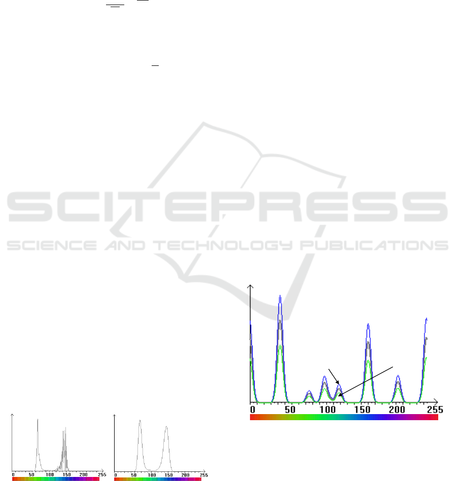
High Threshold

Low Threshold

(a)

ANIT 2023 - The International Seminar on Artiﬁcial Intelligence, Networking and Information Technology

Out of tolerance part

0 50 100 150 200 255

Target image

High Threshold

Low Threshold

(b)

Figure 5: Tone histogram threshold diagram and out of

tolerance diagram.

Figure 5 (a) is a schematic diagram of the high

and low threshold values of the hue histogram when

the percentage deviation between the upper and

lower parts is 30. The advantage of calculating the

high and low threshold through the percentage of

upper and lower deviations is that it takes into

account the inherent frequency of a certain color

tone in the template image, that is, the allowable

deviation of a higher frequency color tone is

relatively large, as shown in Figure 5 (a).

Set the hue histogram of the target image as

𝐻



(𝑘), the number of out of tolerance tones can be

calculated using the following formula:

𝑁 =

∑

Count𝐻



(𝑘)<





HThr

low

(𝑘) 𝑂𝑅 𝐻



(𝑘)>HThr

(𝑘);

(

11)

Among them, 𝑁 represents the number of out of

tolerance tones. Count(⋅) represents a counting

function, 1 is counted when the conditions in

parentheses are met, otherwise 0 is counted.

Figure 5 (b) is a schematic diagram of the color

tone histogram out of tolerance. From it, it can be

seen that the target image has a difference in blue

and green tones.

In summary, the overall process of the color

detection algorithm is shown in below, which mainly

includes:

Step 1. ROI Editing Tool: used to define ROI

regions. If there is no ROI region definition, color

detection is directly performed on the entire image.

Step 2. Color Space Conversion: Transfer the

RGB color space of the image to the HSI color space.

Step 3. Generate Initial Tone Histogram:

Generate an initial tone histogram based on H, S

components, and saturation thresholds.

Step 4. Initial Tone Histogram filtering:

construct a Gaussian filter according to the half

width of the filter and filter and smooth the initial

tone histogram.

Step 5. Generate Hue Histogram Threshold:

Based on the percentage of upper and lower

deviations, generate the template image hue

histogram high and low thresholds.

Step 6. Measurement of Hue Histogram

Difference: Compare the hue histogram of the target

image with the high and low threshold of the

template image hue histogram, and count the

number of out of tolerance hues.

Step 7. Detection Result Judgment: If the

number of out of tolerance tones is greater than the

given threshold, the image color is judged to be out

of tolerance and the out of tolerance tone

information (standard value and out of tolerance

amount) is returned; Otherwise, it is judged that the

image color is not out of tolerance.

5 EXPERIMENTAL DESIGN AND

ANALYSIS

5.1 Applicability Evaluation

The applicability mainly refers to the applicability of

color detection tools to various applications. Two

sets of experiments were designed to evaluate their

applicability: 1) detecting typical Demo images in

Cognex DIP; 2) Detect offset printing images. The

detection parameters of LLV( Luster Light Vision )

and Cognex are shown in Table 1.

Table 1: Applicability Evaluation Test Parameters.

LLV Cognex DIP

Parameter

Type

Parameter

value

Parameter

Type

Parameter

value

ROI Full graph ROI Full graph

saturation

threshold

saturation

threshold

608

Upper

deviation

percentage

Upper

deviation

percentage

Lower

deviation

percentage

Lower

deviation

percentage

Filter half

width

Smoothing

factor

Over tone

threshold

Over tone

threshold

1)Detect Demo images in Cognex DIP

Figure 6 (a) (b) shows two demo images in Cognex

DIP, with Figure 6 (a) as the template image and

Figure 6 (b) as the target image.

Research on Color Vision Tool Design Based on Detection Algorithms

(a) Template image

(b) Target image

Target image

Figure 6: Demo image and two detection results.

Figure 6 (c) (d) shows the detection results of the

image in Figure 6 (a) (b), where Figure 6 (c) is a

histogram representation of the detection results of

LLV, and Figure 6 (d) is a histogram representation

of the detection results of Cognex. Comparing these

two histogram representations, it can be seen that

both detect that the target image has more green and

less blue compared to the template image, which is

completely consistent with the test image. LLV

detected 46 out of tolerance tones, Cognex detected

46 out of tolerance tones, and the number of out of

tolerance tones was consistent.

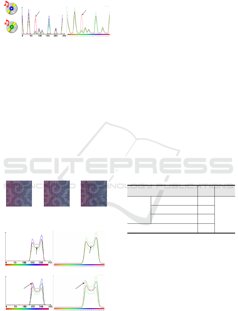
2)Detect Offset Printing Images

Figure 7 shows the offset printing image, where

Figure 7 (a) is the template image, Figure 7 (b) is the

target image 1, which belongs to the same batch of

products as the template image, and Figure 7 (c) is

the target image 2, which is not the same batch of

products as the template image.

(a) Template image

(b) Target image 1

Figure 7: Offset printing image.

(a) Detection result of LLV（Target image 1）

(b) Detection result of Cognex DIP（Target i mage 1）

目标图像

Target image

Figure 8: Detection results of offset printing image.

Figures 8 show the detection results of the

images in Figures 7. For target image 1, LLV

detected 12 out of tolerance tones, while Cognex

detected 9 out of tolerance tones; For target image 2,

LLV detected 48 out of tolerance tones, while

Cognex detected 44 out of tolerance tones. The

number of out of tolerance tones is basically the

same, and the subtle differences are mainly caused

by different histogram filtering strategies, which do

not affect the detection results. For target image 1,

the detection results are all good; For target image 2,

the detection results are all defective products.

3)Efficiency Evaluation

Detection efficiency is also an important focus of

color detection tools. Test the efficiency of color

detection on the images in Figures 7, which image

format is 119×116.

The testing environment is a Pentium 4 CPU

with a main frequency of 2.8GHz, 1GB Byte of

memory, Windows XP operating system, and the

compilation environment is VC6.0 Release version.

Table 2 provides a list of the time required for color

detection by LLV and Cognex respectively. From it,

it can be seen that the time consumption of LLV is

equivalent to that of Cognex DIP.

Table 2: Time consumption for color space conversion

under different high-order byte

bits (ms).

Time consumption list LLV

Cognex

DIP

Sub item

time

consumption

Color Space Conversion 4.03

2.37

Histogram filtering 0.06

Histogram comparison and

out of tolerance detection

0.01

Total time consumption 4.10

6 CONCLUSION

From the aforementioned experiment, the following

basic conclusions can be drawn:

Capable of effective color detection of typical

demo images and offset images in Cognex

DIP;Under equivalent parameter settings, the

number of out of tolerance tones detected by LLV is

basically the same as the number of out of tolerance

tones detected by Cognex DIP. The time

consumption of LLV is equivalent to that of Cognex

DIP.

ANIT 2023 - The International Seminar on Artiﬁcial Intelligence, Networking and Information Technology

REFERENCES

Ma Rui-qing, Liao Ning-fang.Influence of Illuminant

Chromaticity on Color Constancy Under RGB-LED

Light Source[J]. Acta Optica Sinica, 2019, 39(09):418-

426.

Safdar M,Cui G,Kim Y J,et al. Perceptually uniform color

space for image signals including high dynamic range

and wide gamut[J]. Optics Express, 2017,

25(13):15131-15151.

Shamey R,Zubair M,Cheema H.Effect of field view size

and lighting on unique-hue selection using Natural

Color System object colors[J]. Vision Research, 2015,

113: 22-32.

Xiao K,Wuerger S,Fu C,et al. Unique hue data for colour

appearance models. Part I: Loci of unique hues and hue

uniformity[J]. Color Research

＆

Application, 2011,

36(5): 316-323.

Research on Color Vision Tool Design Based on Detection Algorithms