Layered Batch Inference Optimization Method for Convolutional

Neural Networks Based on CPU

Hongzhi Zhao

Xun Liu

Jingzhen Zheng

and Jingjing He

School of Computer and Information Technology, Beijing Jiaotong University, Beijing, China

Zhejiang Scientific Research Institute of Transport, Hangzhou, China

Keywords: Convolutional Neural Network, Batch Processing, Inference Task Scheduling Optimization, CPU.

Abstract: In recent years, CPU is still the most widely used computing system. And in CNN inference applications,

batching is an essential technique utilized on many platforms. The arrival time and the sample number of

the convolutional neural network inference requests are unpredictable, and the inference with the small

batch size cannot make full use of the computation resources of the multi-threading in CPU. In this paper,

we propose a layered batch inference optimization method for CNN based on CPU (LBCI). This method

implements "layer-to-layer" optimal scheduling for being-processed and to-be-processed CNN inference

tasks under the constraints of the user preference delay in a single batch. It conducts the dynamic batch

inference by "layer-to-layer" optimal scheduling during the processing. The experimental results show that

for the request with a single-sample inference task, LBCI reduces the inference time by 10.43%-52.43%

compared with the traditional method; for the request with a multi-sample inference task, LBCI reduces the

inference time by 4.32%-22.76% compared with the traditional method.

INTRODUCTION

Convolutional neural network (CNN) is often used

in the field of computer vision. In practice, since

computer vision tasks such as face recognition (F.

Boutros, 2022), (Kim, 2022) and image

classification (D. Landa-Silva, 2008), (Li, 2023) are

widely applied, the number of CNN deployments are

also showing an increasing trend year by year. CNN

models are deployed on CPU platforms such as

servers, clients, and edge devices for the needs of

some practical applications (Mittal, 2022). In recent

years, CPU is still the most widely used computing

system, and CPU manufacturers continue to launch

CPU products for deep learning applications

(Daghaghi, 2021).

In the cloud server providing the services, the

cloud inference server will process inference

requests sent by users to obtain prediction results. In

most scenarios, a user inference request carries only

one inference sample, which is called a single-

sample inference task; in a small number of

application scenarios, a user inference request

carries multiple inference sample, which is called a

multi-sample inference task (AMAZON, 2018).

Some traditional inference servers can only process

one inference request at a time; some set the

maximum allowed batch size and a batching time

window that is the maximum period time of waiting

for incoming requests to form a batch (Choi, 2021).

With these methods, the server can only process the

tasks in the order of the arrivals. And we call them

as the "end-to-end" coarse-grained inference

method. The "end-to-end" coarse-grained inference

method will produce the good effect under the strict

condition that the batch size of the running inference

tasks is just fit. Actually, the arrival time and the

sample number of the inference requests are

unpredictable. It is hard to form a batch with a fit

batch size all the time for the inference. And it is

also unreasonable to blindly wait the arrival of the

new inference requests to form a batch with a fit

batch size. The running inference tasks with the

small batch size can’t fully utilize the computation

resources of the multi-threading in CPU. After the

running inference tasks are finished, the server needs

to reload the weight data to process the new

inference task. Accessing memory too frequently

will reduce the CPU processing efficiency.

Therefore, the "end-to-end" coarse-grained inference

method is only a suboptimal solution for CPU

platforms.

The related works didn’t provide a solution that

optimizing the inference on CPU while the batch

size is smaller than the ideal value. Based on the

182

Zhao, H., Liu, X., Zheng, J. and He, J.

Layered Batch Inference Optimization Method for Convolutional Neural Networks Based on CPU.

DOI: 10.5220/0012277100003807

Paper published under CC license (CC BY-NC-ND 4.0)

In Proceedings of the 2nd International Seminar on Artiﬁcial Intelligence, Networking and Information Technology (ANIT 2023), pages 182-189

ISBN: 978-989-758-677-4

above, we propose a layered batch inference

optimization method for convolutional neural

networks based on CPU referred to as LBCI. This is

a fine-grained inference method, which converts the

traditional "end-to-end" inference method into a

"layer-to-layer" inference method. The user

preference delay on the server is the most significant

constriction for processing the inference requests.

Hence, LBCI will schedule the to-be-processed

inference task samples to be batching processed with

the being-processed inference task samples in a

running thread within the user preference delay,

while the batch size of the being-processed inference

task samples is smaller than the ideal value. LBCI

can make full use of the parallel capability of the

CPU and improve the average throughput of the

inference server within the user preference delay.

Our contributions can be summarized as follows.

•Our study indicates that the batch process

schedule of the CNN inference on CPU can be

optimized at the level of the layers, not only at the

level of the model. And we design a novel strategy

for predicting the running time with the new batch

size by using the running time ratio lookup table of

the computed sub-models.

•We propose a layered batch inference

optimization method for convolutional neural

networks based on CPU referred to as LBCI which

makes full use of the parallel capability of the CPU

and improve the average throughput of the inference

server within the user preference delay.

RELATED WORK

2.1 Optimizing CNN Inference Task

Scheduling

On homogeneous devices, the focus of scheduling

optimization is fully utilizing resources on the

device; while on heterogeneous devices, the focus of

scheduling optimization is often the division of

computing tasks and communication between

heterogeneous devices. Here we only focus on

research work on scheduling optimization of CNN

inference requests on homogeneous devices. Choi et

al. (Choi, 2021) proposed a batch processing system

LazyBatching that supports SLA (service level

agreement) on the NPU simulator. It performs

scheduling and batch processing at the level of

nodes in the graph, rather than at the level of the

entire graph, and improves the throughput of batch

processing on the NPU simulator. But this work is

based on the NPU simulator, not the CPU platform.

Zhang et al. (Y. Zhang, 2022) proposed a CNN task

scheduling paradigm, "One-Instance-Per-x-Core",

which improved the throughput of multi-core CPU

batch processing on DNN training and inference

tasks. Since ParaX works mainly for DNN model

training, they mainly consider the impact of the

batch size in each instance on the accuracy of the

training results, not on the delay and throughput of

multi-core CPUs. Wu et al. (X. Wu, 2020) proposed

Irinan online scheduling optimization strategy on the

GPU platform for multiple different DNN models’

inference, which reduces delays under unpredictable

workloads, effectively shares GPU resources and

minimizes average inference delays. Irina focuses on

scheduling optimization between different DNN

model inference tasks.

2.2 Using CPU Multithreading to

Calculate CNN Inference Tasks

The CPU computing modules in mainstream deep

learning frameworks such as PyTorch already

support multi-threading technology. The PyTorch

deep learning framework can achieve multiple levels

of parallelism on the CPU platform (Pytorch, 2019).

Liu et al. (Liu, 2019) pointed out that high-

performance kernel libraries (such as Intel MKL-

DNN (INTEL, 2022) and OpenBlas (Zhang, 2016)

are usually used to obtain the high performance of

CNN operations. In the convolution calculation, the

parallel instructions of OpenMP (Openmp] are used

to realize multi-threaded parallel operations at the

same time, making full use of hardware resources

and greatly reduce computing time. Amazon

(Daghaghi, 2021) pointed out that the inference time

per unit image shows a decreasing trend as the

number increases using the MXNet framework on

the CPU platform for CNN inference when the

number of input images is within a certain range.

2.3 Optimizing Batch Processing of

DNN Inference Tasks

Batch research on the inference process of DNN

began in 2018, and Gao et al. (Gao, 2018) firstly

studied the inference process of RNN. The

traditional CNN batch inference method is image-

wise batch processing. Wang et al. (Wang, 2020)

proposed a layer-wise scheduling method on a CPU

processor without parallel optimization. With the

layer-wise scheduling method, the images in one

batch use the weights of one layer at the same time,

reducing the memory accesses and the access delays.

In view of the different weight data and memory

Layered Batch Inference Optimization Method for Convolutional Neural Networks Based on CPU

183

usage of each layer in a CNN model, Choudhury et

al. (

A. R. Choudhury, 2020] proposed a strategy which

used dynamic programming to set the optimal batch

size of each layer of the CNN model on the GPU

platform, making full use of the computational

parallelism of the GPU and speeding up the

inference execution speed.

METHOD

3.1 Overview of LBCI

LBCI consists of four functional modules as shown

in Fig 1: an initialization setting module (IS), a

buffer data storage module (DS), a buffer data

detection module (DD), and a CNN computing

module (CNNC).

Initialization Setting Module: First, LBCI will

run the initialization setting module (IS) on the

corresponding CPU platform to initialize two key

variables and preprocess the CNN model. The key

variables are the user preference delay t

opt

and the

optimal number N

opt

of the batch size for the model

inference. The user preference delay t

opt

is a

hyperparameter provided by the CPU server. We

propose an strategy to calculate the optimal number

opt

with which the running time of the batch

inference must satisfy the constraint of t

opt

. The

strategy is described in the section B.

The IS prepocesses the CNN model at the level of

the layers. As shown in Fig. 2, the IS refers several

sequential convolutional layers as a sub-model and

the whole CNN model can be referred to as a

combination of the sub-models. The preprocess

won’t change the results of the original model.

Based on the sub-models of the CNN model, the

IS runs the model inference to record the running

time of each sub-model. The input data are a batch

of samples and the batch size b is an integer ranging

from 1 to N. The model inference is performed for N

times with the different batch sizes. Then the IS

builds the running time ratio lookup table of the

computed sub-models as shown in Fig. 3. The

running time ratio of the computed sub-models r

p, q

is:

p, q

= ∑t

p, i

÷ t

, (i = 1, 2, …, q)

(1)

where p is the batch size of the input data, q is the

number of the computed sub-models, t

p,i

is the

running time of the sub-modeli with the batch size b

of p and t

is the total running time of the model

with the batch size b of p.

Buffer Data Storage Module: After the

initialization, LBCI uses a thread to independently

run the buffer data storage module (DS) which

receives and stores CNN inference tasks’ samples in

the memory. We define a state variable f for marking

a sample at the being-processed or to-be-processed

state. f = 0 indicates to-be-processed while f = 1

indicates being-processed. The DS maintains a

queue of the samples, in which saves the data, the

arriving time and the state variable f of each sample.

The DS will check all the state variables in the

queue while the new samples arrive, and delete the

samples with f = 1 in the queue. The state variable f

of each new arriving sample is referred to as 0 by

default.

CNN Computing Module: The CNN computing

module (CNNC) loads the preprocessed model

which contains several sub-models. The CNNC with

the certain input data is an instance for the model

inference. One instance needs an individual thread.

Please note that the threads separately running the

different CNNC instances can exist at the same time.

Assuming that the number of the to-be-processed

samples in the queue is N

. If N

≥ N

opt

, the CNNC

instance will read N

= N

opt

to-be-processed samples

from the head of the sample queue and set f = 1. N

is the batch size of the CNNC instance input samples.

And we will not optimize the instance later in the

computing process. If N

< N

opt

, the CNNC instance

will read N

= N

to-be-processed samples and set f

= 1. For the condition, the above CNNC instance can

be optimized in the computing process. Since the

batch size of the instance input data is smaller than

opt

, the purpose of the optimization is increasing the

batch size with the constraint of t

opt

. The CNNC

instance calls the buffer data detection module (DD)

to detect whether it can be optimized or not, when

the calculations of each sub-model are completed as

shown in Fig. 1. Based on the DD’s feedback, if the

CNNC can be optimized, it will continually be

processed in the rest of the sub-models with the

“layer-to-layer” optimal scheduling which is

described in the section D. Once a CNNC instance is

optimized, it will not call the DD and be optimized

again.

Figure 1: The overview of LBCI.

ANIT 2023 - The International Seminar on Artiﬁcial Intelligence, Networking and Information Technology

184

Buffer Data Detection Module: The buffer data

detection module (DD) will count the number N

the to-be-processed samples in the queue after being

called by a CNNC instance. If N

= 0, the DD will

return 0 to the instance, which means that no to-be-

processed sample in the queue. The instance can’t be

optimized at the moment. If N

> 0, the instance can

be optimized. Then the DD utilizes the prediction

strategy to predict how many (N

add

) to-be-processed

samples can be added to the instance while keeping

the total running time will not over t

opt

. And the DD

will return N

add

to the instance. The prediction

strategy is explained in the section C. If N

add

= 0, the

CNNC instance can’t be optimized now and later,

and will never call the DD again. If N

add

> 0, the

CNNC instance will schedule N

add

to-be-processed

inference task samples to be batching processed with

being-processed samples.

3.2 Strategy for Calculating the

Optimal Number N

opt

The strategy calculates N

opt

on the basis of the test

data coming from the multiple inference tests. The

key steps of the strategy are explained as follows.

•The IS runs the model inference for N times with

the different input data batch size b (1 ≤ b ≤ N) and

obtains a set of the average running time per sample

T = {t

} where t

is the average running time per

sample while the batch size is b. Then fitting a

function T = g(b).

•For each batch size b, the inference is performed

for n times. The IS gets a running time set {t

|1 ≤ j ≤

n } and the average running time t

avg

of n inferences

where t

avg

= ∑t

÷ n. And calculating the average

fluctuation ratio r

of the running time per sample by

(2):

= [ ∑ (|t

- t

avg

| ÷ t

avg

)] ÷ n.

(2)

Then we obtain the average fluctuation ratio set

|1 ≤ b ≤ N } and find the maximal ratio r

max

in the

set. Let t

OPT

= t

opt

× r

max

where t

OPT

is the strict user

preference delay.

•With the strict user preference delay t

OPT

, let T =

OPT

and substitut in T = g(b). Then b is obtained

which is the optimal number N

opt

of the batch size

for inference.

3.3 Prediction Strategy of Buffer Data

Detection Module

The prediction strategy produces N

add

being return to

the CNNC instance. Assuming that the CNN model

has x sub-models. The key of the prediction strategy

is that (3) should be valid while N

add

is as large as

possible:

all

= t

wait

+ t

done

+ t

add

+ t

k+1

and t

all

< t

opt

(3)

where t

all

is the predicted total time, t

wait

is the

waiting time for N

add

to-be-processed samples lining

up in the queue, t

done

is the elapsed running time of

being-processed samples in the thread, t

add

is the

predicted running time of N

add

to-be-processed

samples from the sub-model

to the sub-model

(1 <

k < x) and t

k+1

is the predicted running time of (N

add

) samples from the sub-model

k+1

to the sub-

model

. The key steps of the strategy are explained

as follows.

•Initializing N

add

= 1 by default. Since we recorded

the arriving time of the samples in the queue, the DD

can directly calculate t

wait

. And t

done

can be obtained

from the thread running time by calling some system

functions.

Figure 2: The IS refers several sequential convolutional

layers as a sub-model.

Figure 3: The IS builds the running time ratio lookup table

of the computed sub-models.

•Let batch size b = N

add

and substitut in T = g(b),

predicting average running time per sample for b =

Layered Batch Inference Optimization Method for Convolutional Neural Networks Based on CPU

185

add

. In the running time ratio lookup table of the

computed sub-models, the DD finds r

p, q

, (p = N

add

, q

= k). t

add

can be predicted by (4):

add

= N

add

× g(N

add

) × r

p, q

(4)

•Let batch size b = N

+ N

add

and substitut in T =

g(b), predicting average running time per sample for

b = N

add

. In the running time ratio lookup table of the

computed sub-models, the DD finds r

p, q

, (p = N

add

, q = k +1). t

k+1

can be predicted by (5):

k+1

= (N

+ N

add

) × g(N

+ N

add

) × (1 − r

p, q

)

(5)

•Then the DD calculates t

all

by (3). If t

all

< t

opt

add

= N

add

+1 and going back to the step 2. If t

all

≥

opt

, it means that the DD finds the final N

add

at the

sub-model

and ends the prediction. At last, the DD

will return N

add

= N

add

- 1 to the CNNC instance.

3.4 “Layer-to-Layer” Optimal

Scheduling

Assuming that the CNNC instance calls the DD

when the calculations of the sub-model

are

completed. After getting the DD feedback, the

CNNC instance is aware of that N

add

> 0) to-

be-processed samples can be added to the instance

while keeping the total running time will not over t

opt

The specific steps of “layer-to-layer” optimal

scheduling are described as follows.

•The batch processing of N

being-processed

samples in the instance are paused before the sub-

model

k+1

calculations begin. The instance stores N

outputs produced by the sub-model

in the memory.

•The CNNC instance reads N

add

to-be-processed

samples from the head of the queue maintained by

the DS and modifies the state variable f of these

samples to 1. Then the instance processes these N

add

samples in batch from the sub-model

to the sub-

model

and generates N

add

outputs.

•Then the instance loads N

outputs from the

memory and concatenates (N

+ N

add

) outputs

produced by the sub-model

as a new batch. The

new batch will be calculated by the rest of the sub-

models until outputting (N

+ N

add

) results in the

CNNC instance.

EVALUATION

We verify the effectiveness of LBCI in two

perspectives: the effectiveness of strategy for

calculating the optimal number N

opt

and the

comparison with two typical batching inference

methods on the time and throughput. The

verification experiments use AlexNet (Krizhevsky,

2017) as the inference model with the test dataset

ImageNet-2012. We deploy AlexNet by "web

server" method, which is implemented with the

lightweight web framework Flask of Python. The

web page sends the inference requests, and the

backend server receives and responses the requests.

The inference platform is a multi-core CPU platform

with Intel(R) Core (TM) i7-8700 CPU and L1

384KB, L2 1.5MB, L3 12MB.

4.1 Effectiveness of Strategy for

Calculating the Optimal Number

opt

The IS runs the AlexNet inference for N = 256 times

with the different input data batch size b (1 ≤ b ≤

256) and obtains a set of the average running time

per sample T = { t

} where tb is the average running

time per sample while the batch size is b. We

consider that the four-parameter equation fits best.

Then the fitting four-parameter function is:

g(b) = b × [(z1 − z2) ÷ (1+ (b ÷ z3)

) + z2],

(6)

where z1, z2, z3 and z4 are the parameters of the

fitting function.

Then we rerun the AlexNet inference for 100

times with the different input data batch size b (1 ≤ b

≤ 100) and record the real running time per samples

of each time. The real time and the predicted time

calculated by (6) are close as shown in Fig. 4(a),

which preliminarily verifies the effectiveness of (6).

And we calculate the strict user preference delay

OPT

and the optimal batch size N

opt

with (6) on the

basis of the strategy. The running time of performing

the AlexNet inference with b = N

opt

for 100 times is

shown in Fig. 4(b). The blue line denotes that the

user preference delay t

opt

= 500ms. Only 1% of the

inference running time are larger than t

opt

, which

verifies the effectiveness of the strategy for

calculating the optimal number N

opt

4.2 Time and Throughput Comparison

We use two typical batching inference methods to

comprise with LBCI: (1) sequential processing one

task at a time like Amazon Rekognitio inference

server (AMAZON, 2022) referred to as Serial. (2)

Batch processing by setting the maximum allowed

batch size m and a batching time window (Choi,

2021) referred to as Batchsize(m). The web page

sends the requests per second to the backend server

producing four traffics (20/s, 40/s, 60/s and 80/s).

ANIT 2023 - The International Seminar on Artiﬁcial Intelligence, Networking and Information Technology

186

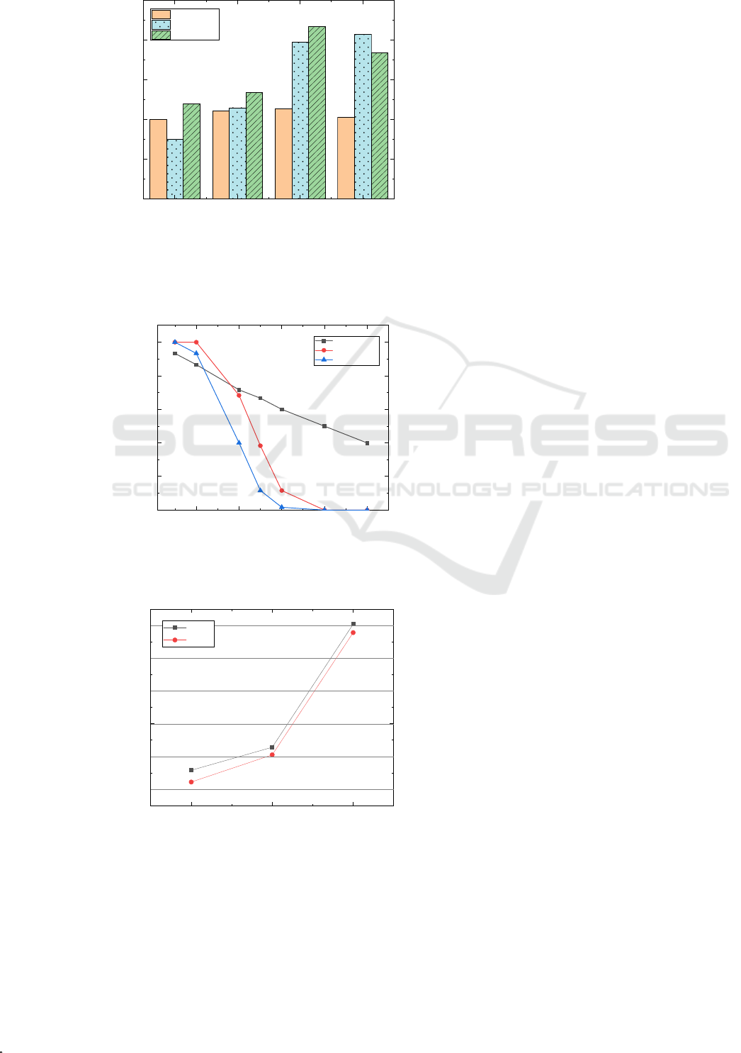
1)The single-sample inference task: The request

with a single-sample inference task is the most

common. The average delay time per batch for LBCI

is always below Serial and Batchsize(10) as shown

in Fig. 5(a). At the low traffic (20/s), the average

delay time per batch for Serial and LBCI is much

less than Batchsize(10). At the medium, high and

heavy traffics (40/s, 60/s and 80/s), since the poor

efficiency of Serial the sequential processing, many

requests are waiting, which causes the larger

increasing of the average delay time per batch for

Serial. With Batchsize(10), the backend server

always processes a batch of the requests after

collecting 10 requests. Therefore, the average delay

time per batch for Batchsize(10) is relatively stable

at four traffics (20/s, 40/s, 60/s and 80/s).

The throughput of LBCI is higher than Serial and

Batchsize(10) at the low, medium and high traffics

(20/s, 40/s and 60/s) as shown in Fig. 5(b). LBCI

sacrifices the throughput for the lower average delay

time per batch at the heavy traffic (80/s). But the

throughput at the heavy traffic (80/s) is still higher

than that at the 20/s and 40/s. At the low traffic

(20/s), LBCI reduces the average delay time per

batch by 26.12% and improves the throughput per

second by 20.3% compared with Serial. At the

medium and high traffics (40/s and 60/s), LBCI

reduces the average delay time per batch by 52.43%

and 19.43%, and improves the throughput per

second by 16.96% and 9.56% compared with

Batchsize(10). Since the average delay time per

batch hardly exceeds the user preference delay t

opt

we only assess the timeout ratio at the high traffic

(60/s), as shown in Fig. 6. The probability for the

average delay time per batch of LBCI exceeding the

user preference delay t

opt

is 11.67% at t

opt

= 500,

which is much lower than Serial and Batchsize(10).

2)The multi-sample inference task: For the

request with a multi-sample inference task, since

Batchsize(m) may divide a request to form a batch of

m samples, it loses the original advantage. Hence, we

compare LBCI with Serial. The web page sends the

requests with num samples per request to backend

server per 100 ms for 10 times. We respectively

conduct three tests to process the num samples and

record the running time of each test. For each test,

num is randomly generated from the different ranges.

The range of [1, 10] means the small data; [1, 25]

means the medium data; [1, 50] means the big data.

As shown in Fig. 7, compared with Serial, LBCI

reduces the running time per test by 22.76% at the

small data, 10.08% at the medium data and 4.32% at

the big data. And the average delay time per batch of

LBCI and Serial is always below the user preference

delay t

opt

at the small data and the medium data. At

the big data, the average delay time per batch of

LBCI occasionally exceeds t

opt

, which can be

accepted. From the analysis results, LBCI is more

suitable for the inference requests

(a)

(b)

Figure 4: (a) Comparison between real time and predicted

time. (b) The running time of performing the AlexNet

inference with b = N

opt

for 100 times.

(a)

20 40 60 80

200

400

600

800

1000

1200

1400

1600

Average delay time per batch (ms)

Number of re

uests

er second

Serial

Batchsize(10)

LBCI

Layered Batch Inference Optimization Method for Convolutional Neural Networks Based on CPU

187

(b)

Figure 5: Comparison between LBCI, Serial and Batchsize

(10) on average delay time per batch and throughput per

second at four traffics (20/s, 40/s, 60/s and 80/s).

Figure 6: The probability for the average delay time per

batch of LBCI exceeding the user preference delay t

opt

. of

the small data and medium data.

Figure 7: The running time of tests for the

small/medium/big data.

CONCLUSION

In the cloud server providing the services, the arrival

time and the sample number of the inference

requests are unpredictable. And the running

inference tasks with the small batch size can’t fully

utilize the computation resources of the multi-

threading in CPU. Based on the mentioned above,

we propose a layered batch inference optimization

method for CNN based on CPU (LBCI). LBCI

executes "layer-to-layer" optimal scheduling for

being-processed and to-be-processed CNN inference

tasks. It conducts the dynamic batch inference by

"layer-to-layer" optimal scheduling during the

processing. The experimental results show that for

the request with a single-sample inference task,

LBCI reduces the inference time by 10.43%-52.43%

compared with the traditional method; for the

request with a multi-sample inference task, LBCI

reduces the inference time by 4.32%-22.76%

compared with the traditional method.

ACKNOWLEDGMENTS

This work was financially supported by Research

and Development Center of Transport Industry of

New Generation of Artificial Intelligence

Technology (202207H).

REFERENCES

F. Boutros, N. Damer, F. Kirchbuchner and A. Kuijper,

ElasticFace: Elastic margin loss for deep face

recognition[C]. 2022 IEEE/CVF Conference on

Computer Vision and Pattern Recognition Workshops

(CVPRW), New Orleans, LA, USA, 2022, 1577-1586.

https://doi.org/10.1109/CVPRW56347.2022.00164.

M. Kim, A. K. Jain and X. Liu, AdaFace: Quality

Adaptive Margin for Face Recognition[C]. 2022

IEEE/CVF Conference on Computer Vision and

Pattern Recognition (CVPR), New Orleans, LA, USA,

2022, 18729-18738. https://doi.org/10.1109/CVPR5

2688.2022.01819.

D. Landa-Silva, K. N. Le, A simple evolutionary

algorithm with self-adaptation for multi-objective

nurse scheduling[J]. Adaptive and multilevel

metaheuristics, 2008, 133-155. https://doi.org/10.

1007/978-3-540-79438-7_7.

Y. Li, W. Liu. Deep learning-based garbage image

recognition algorithm[J]. Applied Nanoscience, vol. 13,

No. 2, 2023, 13(2): 1415-1424. https://doi.org/10.

1007/s13204-021-02068-z.

20 40 60 80

Throughput (imgs/s)

Number of requests per second

Serial

Batchsize(10)

LBCI

200 400 600 800 1000

100

The probability for the average delay time per

batch of LBCI exceeding the user preference delay t

opt

the user preference delay t

opt

(ms)

Serial

Batchsize(10)

HBCI

small data medium data big data

500

1000

1500

2000

2500

3000

Running time per test (ms)

Number of samples per request

Serial

LBCI

ANIT 2023 - The International Seminar on Artiﬁcial Intelligence, Networking and Information Technology

188

S. Mittal, P. Rajput and S. Subramoney, A survey of deep

learning on cpus: Opportunities and co-

optimizations[J]. IEEE Transactions on Neural

Networks and Learning Systems, Oct. 2022, 33(10):

5095-5115. https://doi.org/10.1109/TNNLS.2021.307

1762.

S. Daghaghi, N. Meisburger, M. Zhao, A. Shrivastava,

Accelerating slide deep learning on modern cpus:

Vectorization, quantizations, memory optimizations,

and more[J]. arXiv preprint arXiv:2103.10891, 2021.

https://doi.org/10.48550/arXiv.2103.10891.

AMAZON, Accelerating apache mxnet with the nnpack

library. 2018. Available online. https://aws.amazon.

com/cn/blogs/china/speeding-up-apache-mxnet-using-

the-nnpack-library/.

Y. Choi, Y. Kim and M. Rhu, Lazy batching: An sla-

aware batching system for cloud machine learning

inference[C]. 2021 IEEE International Symposium on

High-Performance Computer Architecture (HPCA),

Seoul, Korea (South), 2021, 493-506. https://doi.

org/10.1109/HPCA51647.2021.00049

A. Krizhevsky, I. Sutskever, G. E. Hinton, ImageNet

classification with deep convolutional neural

networks[J]. Communications of the ACM, 2017,

60(6): 84-90. https://doi.org/10.1145/3065386

Y. Zhang, L. Yin, D. Li, Y. Peng and K. Lu, ParaX:

Bandwidth-Efficient Instance Assignment for DL on

Multi-NUMA Many-Core CPUs[J]. IEEE Transactions

on Computers, Nov. 2022, 71(11): 3032-3046.

https://doi.org/10.1109/TC.2022.3145164.

X. Wu, H. Xu, Y. Wang, Irina: Accelerating dnn inference

with efficient online scheduling[C]. 4th Asia-Pacific

Workshop on Networking, 2020, 36-43. https://doi.

org/10.1145/3411029.3411035

Pytorch, Pytorch chinese tutorial & documentation. 2019.

Available online. https://pytorch.apachecn.org/#/.

Y. Liu, Y. Wang, R. Yu, M. Li, V. Sharma, and Y. Wang,

Optimizing CNN model inference on CPUs[C]. In

Proceedings of the 2019 USENIX Conference on

Usenix Annual Technical Conference (USENIX ATC

'19). 2019, 1025–1040. https://dl.acm.org/doi/10.

5555/3358807.3358895.

INTEL, Intel math kernel library for deep neural networks

(intel mkl-dnn). Available online. https://oneapi-

src.github.io/oneDNN/v0/index.html.

X. Y. Zhang, Q. Wang, W. Saar, et al. Openblas: An

optimized blas library. In Texas Advanced Computing

Center. 2016. Available online. http://www.open

blas.net/.

Openmp, The OpenMP Api specification for parallel

programming. Available online. https://www.

openmp.org.

P. Gao, L. Yu, Y. Wu, and J. Li, Low latency rnn

inference with cellular batching[C]. In Proceedings of

the Thirteenth EuroSys Conference (EuroSys '18).

Association for Computing Machinery, New York,

NY, USA, 31, 1–15. https://doi.org/10.1145/319

0508.3190541.

X. Wang, L. Zhao and P. Li, High throughput cnn

inference and training with in-cache computation[C].

2020 IEEE 38th International Conference on

Computer Design (ICCD), Hartford, CT, USA, 2020,

461-464, https://doi.org/10.1109/ICCD50377.2020.

00084.

A. R. Choudhury, S. Goyal, Y. Sabharwal and A. Verma,

Variable batch size across layers for efficient

prediction on cnns[C]. 2020 IEEE 13th International

Conference on Cloud Computing (CLOUD), Beijing,

China, 2020, 435-444, https://doi.org/10.1109/CLOUD

49709.2020.00065.

Layered Batch Inference Optimization Method for Convolutional Neural Networks Based on CPU

189