Research on Sales Forecast of Fresh Food Industry Based on

ARIMA: Transformer Model

Xiaoli Zhang

, Huailiang Zhang

, Yanyu Gong

, Xue Zhang

and Haifeng Wang

Linyi University, Linyi, China

Xinfa Group, Liaocheng, China

Keywords: Transformer, Time Series, Sales Forecast, Fresh Food.

Abstract: In addition to its high perishability, fresh food also has a strong timeliness. In order to reduce costs and

improve efficiency, it is necessary for enterprises to accurately predict the sales volume of fresh food. This

paper examines how order planning and production output are out of balance in the sales process of fresh food

industries, and presents a time series high-frequency trading big data forecasting model based on the ARIMA-

Transformer combined forecasting model, along with a quantitative analysis of the MAPE and RMSPE

evaluation indexes. Based on the experimental results, the MAPE of the ARIMA-Transformer forecasting

model is 0.171 percent lower than the MAPE of the LSTM, ARIMA, and Transformer models, and the

RMSPE is 0.306 percent lower than that of the LSTM model, proving its rationality and superiority in

predicting fresh food sales volumes.

1 INTRODUCTION

Nowadays, fresh food is produced and sold in a non-

standardized manner. Perishability and timeliness are

important characteristics, and the sale of fresh food is

closely related to timeliness. Using the high-

frequency trading data, a sales forecasting model is

developed using machine learning theory to predict

the sales of various fresh foods based on the changing

law of sales volume in the fresh food industry.

Dynamic scheduling of production plans can be

achieved based on the dynamic distribution of order

quantities by sales portrait, enabling enterprises to

develop logistics distribution and sales strategies,

optimize resource allocation, reduce costs and

increase productivity.

2 RELATED WORK

The prediction accuracy of traditional models is

difficult to meet the needs of major industries.

According to the characteristics of fresh vegetables,

Lu Wang (Lu Wang, 2021) proposed to improve the

support vector machine model by combining the

fuzzy information granulation method and the

optimized particle swarm optimization algorithm, but

considering the limited factors affecting the sales

volume, it could not be effectively solved when

dealing with the uncertain problem. To improve the

accuracy of retail sales forecasting, Huo Jiazhen (Huo

Jiazhen, 2023) and others developed a model based

on Ensemble Empirical Mode Decomposition

(EEMD), Holt-Winters, and Gradient Lifting Tree

(GBDT). Experimental results indicate that the model

has good predictive performance for multi-step

predictions. However, the model needs a lot of data

for training, so it cannot be applied to applications

with small data sample size. Xu Yingzhuo (Xu

Yingzhuo, 2023) and others established a game sales

forecasting model based on the gradient boosting

decision tree (GBDT) algorithm. The experimental

results show that this model has higher goodness of

fit than other forecasting models. However, the model

does not consider the influence of external factors on

sales volume, and the application scenario is

relatively simple.

3 RESEARCH CONTENT

An ARIMA-Transformer model based on time series

data is presented in this paper. There are two main

parts to the model: ARIMA and Transformer. By

combining ARIMA model predictions with

Transformer model predictions, further predictions

Zhang, X., Zhang, H., Gong, Y., Zhang, X. and Wang, H.

Research on Sales Forecast of Fresh Food Industry Based on ARIMA-Transformer Model.

DOI: 10.5220/0012284800003807

Paper published under CC license (CC BY-NC-ND 4.0)

In Proceedings of the 2nd International Seminar on Artiﬁcial Intelligence, Networking and Information Technology (ANIT 2023), pages 397-400

ISBN: 978-989-758-677-4

397

can be made. As the research object of this

experiment, sales data of livestock products in the

slaughter industry are examined. By modeling and

forecasting time series with ARIMA, a data set is

obtained that is recorded as D

. This model

transforms data set Da and data set D

into data sets

in a <Source, Target> format, which is used as input

for the Transformer model to model and predict, as

well as to calculate the MAPE and RMSPE

evaluation indexes.

4 SYSTEM MODEL

LSTM is chosen as an important benchmark model in

this experiment, but its principle is not discussed in

detail.

Figure 1. ARIMA-Transformer Model Structure Diagram.

An ARIMA-Transformer combined forecasting

model is proposed in this paper to further improve the

accuracy of fresh food sales forecasts. According to

Fig. 1, the structure of the overall model is divided

into three parts: ARIMA, Time-Series-Transformer,

and Time-Series-Transformer-ARIMA. ARIMA and

the improved Transformer model are combined in this

model.

4.1 Data Preprocessing

Figure 2. Data preprocessing step diagram.

According to Fig. 2, the collected sales order data are

classified into sales orders according to meat names,

and the customer's order data are randomly selected

as the experimental data set, which mainly includes

two columns: Date and Value. In the experiment, the

data set is divided into training and test sets in a ratio

of 8:2 chronologically.

4.2 Based on ARIMA Sales Forecasting

Model Design

In the ARIMA(p,d,q) model, 







 stands for

difference operation and stands for the number of

differences required when transforming time series

into stationary series:

















 







  (1)

In the model 







, the number of autoregressive

terms is p, and 







is the autoregressive model.

The formula includes 



as the current value, 



the error term,  as a constant, and 



as the

autocorrelation coefficient. In particular, the formula

is as follows:





 















 



(2)

MA(q) is a moving average model in which 



stands for white noise,  is a constant, and 



is a

coefficient of autocorrelation. In particular, the

formula is as follows:





 















 



(3)

4.3 Based on Transformer Time Series

Sales Forecasting Model Design

The decoder is modified to make it possible to predict

time series data using the traditional Transformer

model. Compared with the traditional Decoder part,

the <Source, Target> sequence of sales volume is

generated based on the sliding window, and most of

the data for Target is derived from the Source, so it is

not necessary to add attention mechanisms on the

Target side. Therefore, the Decoder part keeps only

the full connection layer of the connection system.

Fig. 3 shows the specific structure.

Figure 3. Time-Series-Transformer Model.

In this model, the time series data set is changed

to the form of <Source, Target> in the form of sliding

window, where the sliding window period is 15, i.e.

input_window=15 and output_window=1, so the past

15 days' sales data are used to predict the next day's

sales data.

ANIT 2023 - The International Seminar on Artiﬁcial Intelligence, Networking and Information Technology

398

4.4 Based on ARIMA and Transformer

Combination Forecasting Model

Design

As shown in Fig. 1, the real data set Da is taken as the

input to the Time-Series-Transformer model, and the

prediction result D

from the ARIMA model is taken

as the label value. Based on the Time-Series-

Transformer model and ARIMA, the data set Da is

used as input, along with the other parameters that are

consistent with those in Section 3.3.

5 EXPERIMENT AND RESULT

ANALYSIS

5.1 ARIMA Model Construction

The ARIMA model is one of the most commonly used

time series prediction models. Based on the premise

that the data should be stable, it is necessary to make

one or more differential treatments on the unstable

data, which depends on the value of parameter d in

ARIMA(p,d,q). Most of the time series data are

unstable, so it is necessary to make one or more

differential treatments on the unstable data.

Figure 4. Timing diagram of livestock product sales.

Based on timing Fig. 4, the overall sales volume

of the product is stable and wireless. In order to

confirm whether the data set is stationary, we do ADF

test, and the results show that the p values of the

original data and the first-order difference are close to

0, which meets the stationarity condition. In order to

compare the prediction results with other models, we

make a first-order difference between the data sets,

that is, d=1.

Table 1. ADF test results.

Origin Value

First Difference value

Test Statistic Value

-5.865557

-9.066090

p-value

3.332044x10-7

4.428753x10-15

Number of Observations Used

408

398

Critical Value(1%)

-3.446479

-3.446887

Critical Value(5%)

-2.868650

-2.868829

Critical Value(10%)

-2.570557

-2.570653

In order to determine the values of parameters p

and q in ARMA (p, d, q), the Bayesian Information

Criterion (BIC) is used as the standard. According to

Fig. 5, the square with the minimum BIC is in the

square of AR

and MA

, i.e., the parameters p=0 and

q=1, so ARIMA(0,1,1) is used to model the dataset.

Figure 5. BIC thermal diagram.

Fig. 6 illustrates the prediction result of

ARIMA(1,1,1) on the complete dataset. According to

the figure, the prediction result obtained using the

ARIMA model is very close to the real data, with

MAPE of 1.815 and RMSPE of 3.301.

Figure 6. ARIMA model prediction result diagram.

5.2 Construction of Combined

Forecasting Model Based on

ARIMA and Transformer

In Section 3.3, the ARIMA-Transformer model is

discussed. Based on the prediction results shown in

Fig. 7, MAPE is 1.644, and RMSPE is 2.995.

Research on Sales Forecast of Fresh Food Industry Based on ARIMA-Transformer Model

399

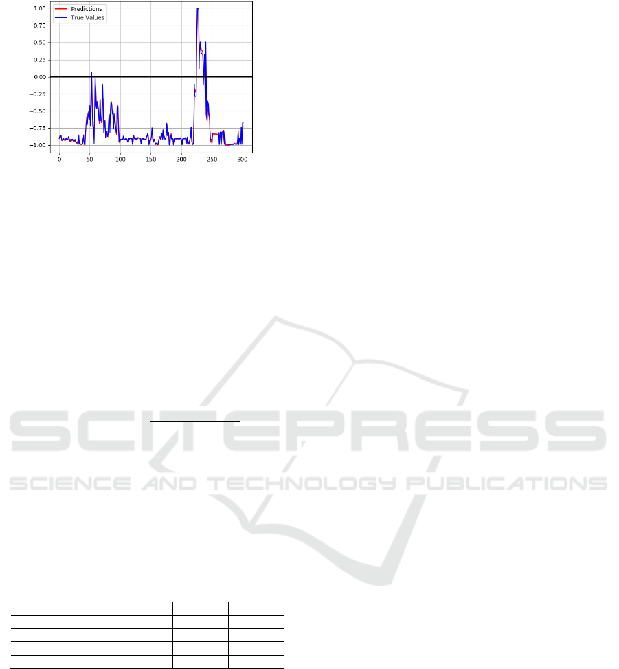
Figure 7. ARIMA-Transformer Model Prediction Result

Diagram.

5.3 Performance Evaluation Indicators

We evaluate the prediction results using Mean

Absolute Percentage Error (MAPE) and Root Mean

Square Percentage Error (RMSPE). A detailed

calculation formula can be found below: (where y

the sample's real value at time i, y is its predicted

value at the current time, x_min is its minimum value,

x_max is its maximum value, and m is its length).

（1） Mean absolute percentage error (MAPE)















 





 







(4)

（2） Root mean square percentage error (RMSPE)



















 





 









(5)

In Table 2, we compare the forecast results of the

fresh food industry using the ARIMA-Transformer

model with other models. In the ARIMA-Transformer

model, the error between the predicted value and the

real value is the smallest, with a reduction in MAPE

by 0.17051 and 0.30604 respectively, and a relatively

high overall performance.

Table 2. Model Evaluation Indicators

MODEL

MAPE

RMSPE

LSTM

4.87734

8.12778

ARIMA

1.81493

3.30136

Time-Series-Transformer

4.57646

ARIMA-Transformer

1.64442

2.99532

6 CONCLUSION

It presents a ARIMA-Transformer forecasting model

for time series high-frequency trading big data,

addressing the imbalance between order planning and

production output in the fresh food industry's sales

process. Experiments show that the prediction results

of this model are more accurate than other models,

thus helping enterprises to better optimize supply

chain management and adjust production.

ACKNOWLEDGEMENTS

This project is supported by Shan dong Province

Science and Technology Small and Medium

Enterprises Innovation Ability Enhancement Project

of China (No. 2023TSGC0449)

REFERENCES

Shi Jiannan, Zou Junzhong, Zhang Jian, et al. Research on

stock price time series prediction based on DMD-LSTM

model (J). Computer Application Research, 2020,

37(3):5.

Lu Wang. Study on the forecast of the sales trend of fresh

vegetables based on improved SVM (D). Anhui

Agricultural University, 2021.

DOI:10.26919/d.cnki.gannu.2021.000101.

Huo Jiazhen, Xu Jun, Chen Mingzhou. Multi-step forecast

of retail sales based on EEMD-Holt-Winters-GBDT

model (J/OL). Industrial Engineering and Management:

1-14 (June 30, 2023). http://kns.cnki.net/kcms/detail/.

Xu Yingzhuo, Guo Bo, Wang Liupeng. Research on game

sales forecasting model based on GBDT algorithm (J).

Intelligent Computer and Application, 2023,

13(01):182-185.

Mostafa M,Zahra A,Poneh Z, et al. Time series analysis of

cutaneous leishmaniasis incidence in Shahroud based on

ARIMA model(J). BMC Public Health, 2023, 23(1).

Atul S, Kumar P J. A multi-model forecasting approach for

solid waste generation by integrating demographic and

socioeconomic factors: a case study of Prayagra j, India

(J). Environmental monitoring and assessment, 2023,

195(6).

Muriithi B M,Samuel W. Time Series Analysis and

Forecasting of Household Products’ Prices (A Case

Study of Nyeri County)(J). Mathematical Modelling and

Applications, 2023, 7(2).

Yuhong J,Lei H,Yushu C. A Time Series Transformer based

method for the rotating machinery fault diagnosis (J).

Neurocomputing, 2022, 494.

Shengchun P,Xian Y,Qianqian L, et al. Time series

prediction of shallow water sound speed profile in the

presence of internal solitary wave trains(J). Ocean

Engineering, 2023, 283.

Liyanage D R. Inflation Forecasting Using Automatic

ARIMA Model in Sri Lanka (J). International Journal

of Economic Behavior and Organization, 2023, 11(2).

ANIT 2023 - The International Seminar on Artiﬁcial Intelligence, Networking and Information Technology

400