Prediction of GGDP Based on SEEA-2012 and Logistic Model

Min Chen

, Jie Shen

, Yun Wu

and Tianhong Zhou

Wuhan Business University, Wuhan, China

Wuhan Polytechnic, Wuhan, China

Keywords: GGDP, SEEA-2012, Logistic Model, BP Neural Network Model.

Abstract: The traditional GDP cannot understand the ecological damage and environmental pollution in the process of

development, so it cannot really show the real situation of a country's economy, so in order to measure the

true economic health of a country, taking into account environmental factors, the GGDP was proposed. In

this paper, SEEA-2012 accounting method is chosen, three indexes which affect GGDP are selected, and the

indexes which affect GGDP are queried and calculated by SEEA-2012 accounting method, using the

Logistic model to forecast the data of natural capital in 2012-2021, using natural capital consumption data

and global temperature data to establish the BP neural network model to forecast the global temperature,

compared with the actual global temperature, the change of temperature was slowed down, and the stability

of the model is judged to be good by sensitivity analysis after adding GDP factors.

1 INTRODUCTION

There are three forms of expression of GDP,

namely, value form, income form and product form

(Wu Nan， 2007). the current method of calculating

GDP is based on the three forms of expression of

GDP, its methods are: production method, income

method and expenditure method.

Traditional GDP accounting has its drawbacks:

not all production is included in GDP, and “GDP”

does not take into account the effect of inflation on

the currency. GDP is not a measure of a country's

overall standard of living or happiness. “Although

changes in per capita gross domestic product are

often used to measure whether the average citizen of

a country is doing well or badly, they do not include

things that might be considered important for

general well-being(Callan, T., 2023).

The System of Integrated Environmental-

Economic Accounting (SEEA) was created in the

1980s from the concept of sustainable development.

It is based on the SNA-1993, a set of accounts built

in cooperation with international organizations (Hoff

Jens V, 2020) there is a strong correlation between

SEEA and SNA.

In this paper, SEEA-2012 accounting natural

capital is classified as natural resource depletion

value cost, environmental pollution damage value

cost and ecological benefit improvement value. In

accounting for this natural capital, the consumption

and unit price of each indicator are looked for, and

each data has a relevant source, and the relevant

calculation formula is used for each indicator, the

resulting GGDP is closer to the real thing. Because

GGDP is a measure that has emerged in recent

years, the SEEA-2012 accounting system used in

this article was adopted by the United Nations after

the 2012 revision of the SEEA accounting system

theory, governments and academics use the system

to account for GGDP after 2012. To better find these

indicators, this paper selects the period from 2012 to

2021. In this paper, a comprehensive and unified

accounting method for natural resource depletion,

environmental pollution damage and ecological

benefit improvement is established, which fully

combines the latest research results and is consistent

with the theoretical framework, in line with

increasingly stringent environmental constraints and

policies.

2 RESEARCH HYPOTHESES

Considering that many of the GGDP-related data are

available internationally in U.S. dollars, in order to

better understand these indicators, the US dollar

settlement unit at the direct exchange rate of

1.00USD: 6.8CNY into RMB. Considering also that

GGDP is the main indicator of a country's economic

health, countries will change their behavior because

474

Chen, M., Shen, J., Wu, Y. and Zhou, T.

Prediction of GGDP Based on SEEA-2012 and Logistic Model.

DOI: 10.5220/0012286200003807

Paper published under CC license (CC BY-NC-ND 4.0)

In Proceedings of the 2nd International Seminar on Artiﬁcial Intelligence, Networking and Information Technology (ANIT 2023), pages 474-482

ISBN: 978-989-758-677-4

of this way of assessing and comparing economies,

thus having a good effect on the natural

environment, that is, an increased blocking effect.

So in order to fully analyze the problem and

simplify the model, we make the following

reasonable assumptions.

Hypothesis 1: It is assumed that when looking for

categories of consumption of natural capital, the

estimated data are meaningful due to the difficulty

of measuring the data.

Hypothesis 2: The conversion of United States

dollars into renminbi is assumed to be free of the

effects of inflation and exchange rate changes.

Hypothesis 3: Suppose that the human-induced

change in the consumption of natural capital from

the original exponential curve to a restricted Logistic

curve, that is, the consumption of natural capital

increases to a certain amount after the growth rate

will decline.

3 DATA SOURCES AND MODEL

DESIGN

3.1 Data Sources

Based on global temperature, GDP and worldwide

consumption of various resources from 2012-2021,

we choose a method that can mitigate climate

change in the calculation of GGDP, and measure and

calculate the global impact of GGDP, estimate how

this global impact will mitigate climate change. The

global average temperature and global GDP in this

paper were obtained from World Bank Open Data |

Data, and the worldwide consumption of various

resources was obtained from World Health Data

Platform (who.int), World Meteorological

Organization | (wmo.int) and World Bank Open

Data | Data.

3.2 Modeling

1) SEEA-2012 Analysis of Accounting for The

Depletion Value of Natural Capital

SEEA-2012 classifies the value of natural capital

depletion into the cost of natural resource depletion,

the cost of environmental pollution damage and the

value of ecological benefit improvement (Yiu Lee

Fai, 2017). The formula is as follows:

(1)

Among them, is the consumption

of natural capital, is the cost of

reducing the value of natural resources,

is the cost of environmental pollution

damage, and is the value of

improving ecological benefits.

The depletion value cost of natural resources

focuses on the quantitative aspects of the utilization

of natural assets, including the material flows and

sources of utilization of resources in economic

processes, and on the quantity of resource depletion

and its efficiency in the process of exploitation and

utilization, resources include water resources, energy

minerals, forest resources and land resources. The

formula is as follows:

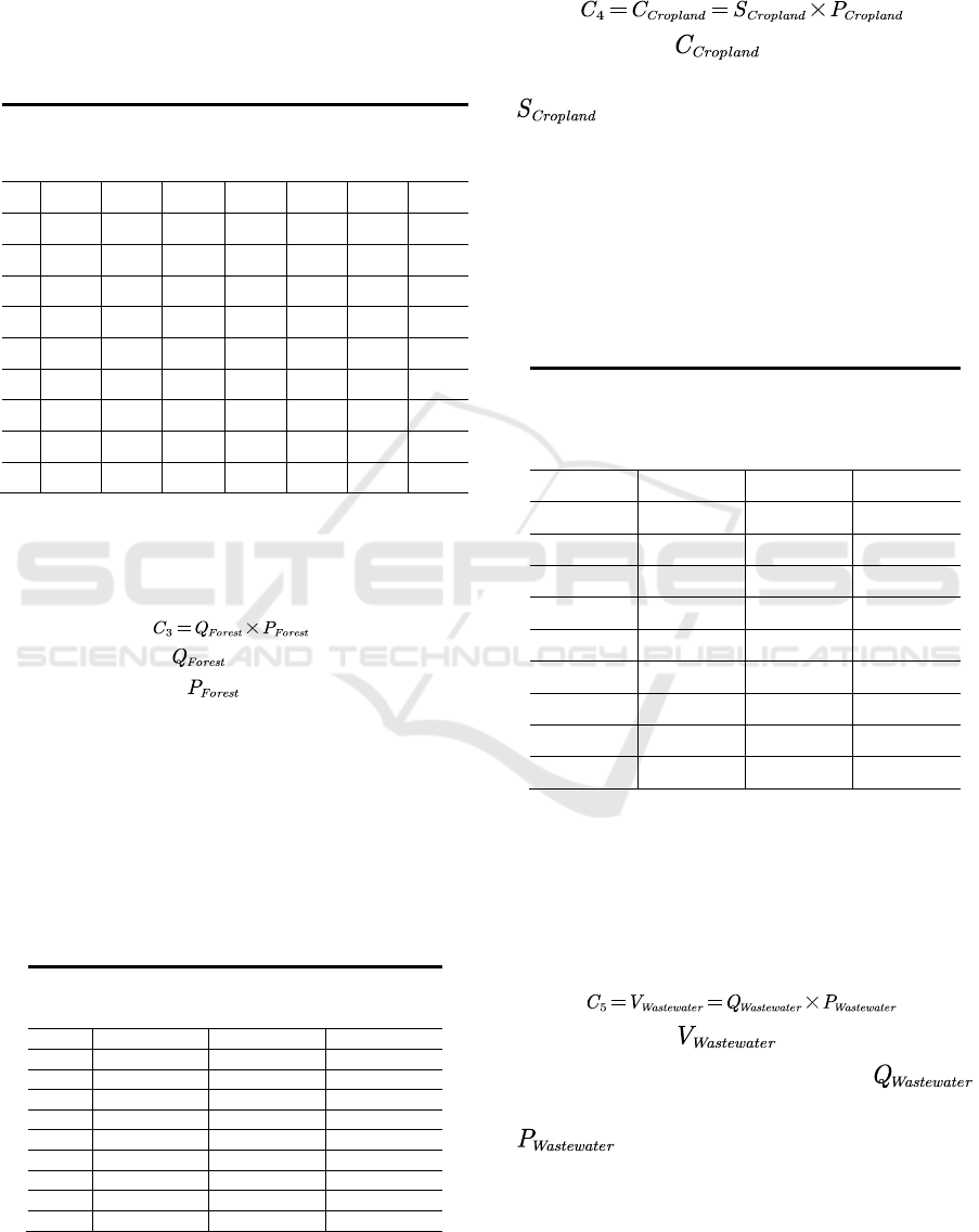
(2)

Among them, is the cost of

reducing the value of natural resources, is the

cost of reducing the value of water resources, is

the cost of reducing the value of energy minerals,

is the cost of reducing the value of forest

resources and is the cost of reducing the value

of land resources.

Environmental pollution damage accounting

includes true object and value cost accounting of

pollutants (water and air pollution). The formula is

as follows:

(3)

Among them, C

is the cost of water resources

rectification, C

is the cost of air pollution control.

Ecological benefit accounting is mainly

accounting for the quality of services and their value

costs of various ecosystems, represented by

conservation soil values. The formula is as follows:

(4)

Among them, is the value of

ecological benefit improvement, is the

value of soil consolidation, and is the

value of fertilizer conservation.

2) The Principle and Calculation Formula of The

Logistic Model

The Logistic model is derived from the

exponential growth model, that is, the classification

index of the value of natural capital depletion is

regarded as the continuous differentiable function

x(t) of continuous time t. The value of each category

index at the initial time (t =0) is x

. Suppose that the

growth rate per unit time is a constant r,

Prediction of GGDP Based on SEEA-2012 and Logistic Model

475

is the growth of x(t) per unit time, the

differential equation and initial conditions satisfied

by x(t) are thus obtained as follows(Ji Yancui,

2014):

(5)

Get the logistic model:

(6)

The parameter solution is consistent with the

above exponential growth model method, requiring r

and .

3) The Basic Principle of 3BP Neural

Network

A neural network model consists of a number of

neurons linked by adjustable connection weights.

Each neuron multiplies the initial input value by a

certain weight and adds other inputs into the neuron,

finally, a sum is calculated, and the output value is

normalized by the excitation function after the

deviation adjustment of the neuron (Zhao Jian,

2016).

First, we initialize the link weights W

and W

usually using the random initialization method. In

the general linear regression fitting process, we

always add a bias b, the offset items b

and b

are

added to the input layer and the hidden layer

respectively, and the following formulas are

obtained:

(7)

Then, add a nonlinear activation function F to the

hidden layer and the output layer to get:

(8)

After outputting Y, a forward propagation is

completed, followed by a backward propagation,

and the backward propagation information is the

error, that is the network output value Y and the true

value of the gap. This difference is usually

expressed by the mean square error loss function,

and the resulting mean square error loss function is

as follows:

(9)

The smaller the error is, the closer the network

is to the real relationship. BP neural network training

can greatly solve the training efficiency problem.

4 EMPIRICAL ANALYSIS

4.1 SEEA-2012 Accounts for the

Depletion of Natural Capital

1) Depletion of Natural Resources

a) Accounting for The Cost of Water Depletion

Value

Access to United Nations databases and the

official website of the World Resources Institute and

other authoritative websites provides information on

the amount of water used worldwide each year.

Based on a large amount of information and the

trend of water price changes, this topic sorted out the

2012-20212021 price. After obtaining the global

water consumption and price, we calculated the

2012-2021 water resource value cost data as follows:

Table 1: Global Water Resources Depletion Value Cost

Table 2012-2021.

Year

Water consumption

(cubic meters)

Water Price

(cubic

meters/yuan)

Water depletion

value cost (million yuan)

2012

5694700000000

8.4

478354800

2013

6054800000000

8.6

5207128000

2014

6248900000000

9.1

5686499000

2015

6548600000000

9.3

6090198000

2016

6493500000000

9.8

6363630000

2017

6832500000000

10.1

6900825000

2018

7126800000000

10.6

7554408000

2019

7265900000000

10.8

7847172000

2020

7625900000000

11.2

8541008000

2021

8269400000000

11.6

9592504000

b) Accounting for The Cost of Reducing The Value

of Energy Minerals

The formula for calculating the cost of energy

and mineral depletion is as follows:

(10)

Among them, is energy mineral

consumption (10,000 tons), is energy

mineral price (10,000 yuan/10,000 tons), is the

main category of energy minerals. Inquiring about

global energy mineral consumption, the

International Energy Agency (IEA) was selected,

and based on the trend of energy prices, the price of

coal was 651,255 yuan per ton, while the price of oil

was 539 yuan per barrel, or 39,340 yuan per ton,

natural gas costs 3.8 yuan per cubic meter, or 5,510

yuan per ton, gasoline 15,000 yuan per ton, diesel

ANIT 2023 - The International Seminar on Artiﬁcial Intelligence, Networking and Information Technology

476

12,000 yuan per ton, and clean energy 8,000 yuan

per ton, combined with formula 10, the global

consumption values of energy minerals and the cost

of energy mineral depletion are calculated as

follows:

Table 2: Table of consumption values of various minerals

and cost tables of energy mineral depletion values.

Year

Coal

consumptio

n value

(million

yuan)

Oil

consumptio

n value

(million

yuan)

Consumptio

n value of

natural gas

(million

yuan)

Gasoline

consumptio

n value

(million

yuan)

Diesel

consumptio

n value

(million

yuan)

Clean

consumptio

n value

(million

yuan)

Cost of

energy

mineral

consumptio

n (million

yuan)

2012

88661.84

6312857.34

627486.24

524113.04

486376.89

236044.98

8275540.33

2013

89856.16

6397894.65

635938.79

531173.10

492928.63

239224.62

8387015.95

2014

91519.82

6516349.79

647713.01

541007.61

502055.06

243653.80

8542299.08

2015

92416.57

6580200.03

654059.60

546308.66

506974.43

246041.23

8626000.51

2016

93246.99

6639326.98

659936.71

551217.56

511529.89

248252.05

8703510.19

2017

94502.68

6728733.90

668823.59

558640.40

518418.29

251595.08

8820713.93

2018

96229.22

6851665.97

681042.81

568846.61

527889.64

256191.65

8981865.90

2019

98679.74

7026146.78

698385.88

583332.54

541332.59

262715.69

9210593.22

2020

99602.32

7091836.08

704915.27

588786.27

546393.66

265171.89

9296705.49

2021

95341.32

6788446.24

674758.89

563597.90

523018.85

253827.79

8898990.98

c) Accounting for The Cost of Reducing The Value

of Forest Resources

The formula for calculating the cost of the

declining value of forest resources is as follows:

(11)

Among them, is the area of the New

Forest Loss (hm

), is the transfer price of

forest resources (10,000 yuan/10,000 hm

). By

consulting the World Resources Institute and the

Foresight Database website to obtain the annual area

of forest resources and their transfer prices, the

reduced value costs for the period 2012-2021 for

2021 are calculated using Formula 11 after obtaining

the area of New Forest losses and the transfer price,

as follows:

Table 3: The cost of declining value of forest resources.

Year

New Forest Loss

(hm

)

The circulation price

of forest (10,000

yuan/10,000 hm

The cost of reducing

the value of forest

resources (10,000

yuan)

2012

59.8

16.08

961.584

2013

55.7

16.38

912.366

2014

50.6

17.21

870.826

2015

44.9

17.85

801.465

2016

29.8

18.06

538.188

2017

16.4

17.68

289.952

2018

10.3

18.11

186.533

2019

8.5

18.35

155.975

2020

18.68

74.72

2021

19.64

39.28

e) Accounting for The Cost of Declining Value of

Land Resources

The formula for calculating the cost of declining

land value is as follows:

(12)

Among them, is the cost of reducing

the value of cultivated land resources (10,000 yuan),

is the global area of cultivated land (hm

the value of each hm

land (hm

/10,000 yuan).

Access the World Bank website, the World

Resources Institute, and other authoritative sites to

obtain land and arable land area and the value of

each hm

of land. Using formula 12, the cost of

declining value for 2012-2021 can be calculated as

follows:

Table 4: Cost of declining value of land resources.

Year

Global arable

land area

(hm

)

Yield of

arable land

(10,000 yuan/

)

Cost of

declining

value of land

resources

(10,000 yuan)

2012

158834000

1.21

192189140

2013

159132000

1.31

208462920

2014

159281000

1.35

215029350

2015

159371000

1.42

226306820

2016

159434000

1.53

243934020

2017

160026000

1.56

249640560

2018

159817000

1.65

263698050

2019

159579000

1.68

268092720

2020

159348000

1.86

296387280

2021

159237000

1.76

280257120

2) Cost of Environmental Damage

a) Accounting for The Cost of Water Pollution

Rectification

This paper calculates the cost of treatment

required to treat wastewater. The formula for

accounting for the cost of water pollution

rectification is as follows:

(13)

Among them, is the treatment cost

(10,000 yuan) for wastewater treatment,

is the amount of wastewater discharge (10,000 tons),

is the cost of wastewater treatment

(10,000 yuan/10,000 tons). According to the official

website of the World Meteorological Organization,

global wastewater discharge has reached 4,260 m

the past two years. The annual global wastewater

Prediction of GGDP Based on SEEA-2012 and Logistic Model

477

discharge is about 4,000 m

. By default, 1 m

is 1

ton, combined with the trend of global wastewater

discharge, the data required for the study were

collated, and the global wastewater discharge and

wastewater treatment cost prices were obtained.

With formula 13, the 2012-2021 clean-up costs were

calculated as follows:

Table 5: Cost of water pollution rectification.

Year

Discharge

of waste

water

(10,000

tons)

Price

(10,000

yuan/10,000

tons)

Clean-up

of water

pollution

(10,000

yuan)

2012

39246961

1.539

60401073

2013

38846594

2.114

82121700

2014

39517356

2.963

117089926

2015

40686172

3.247

132108000

2016

39557163

3.765

148932719

2017

40715869

4.025

163881373

2018

41695718

4.836

201640492

2019

41865567

5.231

218998781

2020

42175143

6.012

253556960

2021

42605240

6.978

297299365

4.2 Accounting for Air Pollution

Control Costs

The formula for calculating the cost of air pollution

control is as follows:

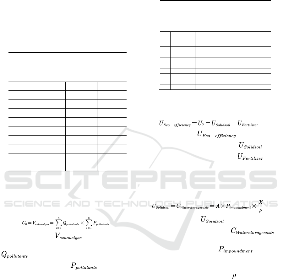
(14)

Among them, is the cost of

controlling pollutants in air pollution (10,000 yuan),

is the amount of major pollutants in the

air (100 million tons) , and is the average

unit treatment price of pollutants (yuan/ton) , n is the

major category of air pollutants. Global average

annual emissions of air pollution between 2010 and

2019 were the highest in human history, reaching 59

billion tones in 2019, a 12% jump from 52.5 billion

tones in 2010, according to the UN report, the

average annual growth rate in the past 10 years was

1.3%. The study data were obtained in conjunction

with global trends in exhaust emissions, the total

cost of air pollution control in the past 10 years was

calculated.

Table 6: The cost of air pollution control and the global

cost of air pollution control.

Year

governance

value cost

(billion

yuan)

Nitrogen

oxide

treatment

value cost

(billion

yuan)

Cost of flue

gas

treatment

value

(billion

yuan)

Total cost of

air pollution

control

(10,000

yuan)

2012

280178.5144

502324.508

88144.69104

8706477134

2013

308611.17

553300.65

97089.65831

9590014783

2014

364550.4187

653592.6215

114688.2519

11328312920

2015

438033.0852

785337.714

137806.0378

13611768370

2016

496699.515

890519.175

156262.6077

15434812980

2017

516686.5704

926353.428

162550.5732

16055905720

2018

587062.112

1052527.84

184690.8518

18242808040

2019

798703.65

1431974.25

251273.6803

24819515800

2020

1035802.68

187062.711

325865.4839

32187308750

2021

1548367.52

2696711.36

473488.62

47185675000

3) Ecological Efficiency Improvement Value

a) Soil Conservation Value

The formula is as follows:

(15)

Among them, is the value of

ecological benefit improvement, is the

value of soil consolidation, and is the

value of fertilizer conservation. The sequestration

value generated by the forest ecosystem can be

calculated by the cost required for water storage,

which is calculated by a specific formula. The

formula is as follows:

(16)

Among them, the value of soil

consolidation (10,000 yuan) , is

the cost of water storage (10,000 yuan) ,A is a new

area of forest (hm

) , and is the cost

of average storage capacity (yuan/m

) ,X is the

annual average reduction of land loss from forested

land to unforested land (t/hm

) , is Represents the

soil capacity contained in the forest (g/cm

). The

annual area of forest resources (hm

) was obtained

by consulting the official website of the World

Resources Institute and the forward-looking

database and other official websites, and the area

added to the forest (hm

) was obtained by subtract

the first from the last, the cost of the average storage

capacity can reach 6.11 yuan per cubic meter, or

6.11 thousand yuan per hectare, and the annual

average reduction of land loss from forested land to

non-forested land is 334.57 tons/hectare, or 33.457

kg/hectare, soil bulk density is 1.24 g/cm

, or 1240

kg/m

. The value of soil consolidation in the last 10

ANIT 2023 - The International Seminar on Artiﬁcial Intelligence, Networking and Information Technology

478

years can be calculated by using the data in Formula

16 as shown in table 7.

The method of calculating the value of fertilizer

preservation is to calculate the three main nutrients

in soil, namely nitrogen, phosphorus and potassium.

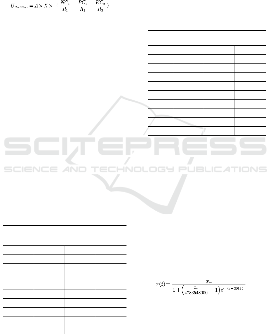
The detailed formula is as follows:

(17)

Among them ,A is the newly increased area of

forest (hm

) ,X is the annual average reduction of

land loss in forested land compared with non-

forested land (t/hm

) , and N is the average nitrogen

content (%) in forest soil, C

is the price of diamine

phosphate fertilizer (yuan/ton) , R

is the content of

nitrogen in diamine phosphate fertilizer (%) , P is

the average content of phosphorus in forest soil (%) ,

is the content of phosphorus in diamine

phosphate fertilizer (%); K is the average potassium

content (%) in forest soil, C

is the price (yuan per

ton) of potassium chloride fertilizer, R

is the

potassium content (%) of potassium chloride.

According to the searching data, the average

nitrogen content, phosphorus content and potassium

content in forest soil were 0.11% , 2.23% and

0.37%, respectively, and the nitrogen content and

phosphorus content in diamine phosphate fertilizer

were 14.0% and 15.0% , respectively, the potassium

content in potassium chloride is 50.0% , the price of

diamine phosphate fertilizer is 2,400 yuan per ton, or

0.24 million yuan per ton, and the price of potassium

chloride fertilizer is 2,200 yuan per ton, or 0.22

million yuan per ton, using the data from Formula

17, the fertilizer retention values for the past 10

years are shown in table 7. Combined with formula

15 for soil conservation values, the final

conservation values are shown in table 7:

Table 7: Soil conservation values.

Year

Soil

consolidation

value (10,000

yuan)

Fertilizer

Value (10,000

yuan)

Soil

conservation

value (10,000

yuan)

2012

-9.86102

- 784.163

-794.024

2013

- 9.18493

-730.4

- 739.585

2014

-8.34394

- 663.523

-671.867

2015

- 7.40401

-588.778

-596.182

2016

-4.91402

-390.77

-395.684

2017

- 2.70436

-215.055

-217.759

2018

-1.69847

- 135.065

-136.763

2019

-1.40165

-111.461

-112.863

2020

-0.6596

- 52.4524

-53.112

2021

- 0.3298

-26.2262

- 26.556

To sum up, water resources, energy and mineral

depletion value, forest resources and land resources,

the cost of reducing value, the cost of cleaning up

water pollution, the cost of cleaning up air pollution,

and the value of soil conservation are added together

to get the cost of natural capital, and then the cost of

GDP minus the cost of natural capital is used to get

the GGDP. See Table 8:

Table 8: Natural capital consumption and GGDP.

Year

Global natural

capital

(10,000 yuan)

Global CDP

(10,000 yuan)

Global GGDP

(10,000 yuan)

2012

13750892643

51340000000

37589107357

2013

15096116071

52774800000

37678683929

2014

17355475038

54216400000

36860924962

2015

20069008589

51129200000

31060191411

2016

22200014163

51992800000

29792785837

2017

23379073874

55352000000

31972926126

2018

26271536771

58792800000

32521263229

2019

33162990163

59602000000

26439009837

2020

41287557823

57874800000

16587242177

2021

57364634542

65694800000

8330165458

4.3 Logistic Model Predicts the

Consumption of Natural Capital

Under Constraints

Because the classification of the depletion value of

natural capital refers to the tendency to change over

time similar to the exponential model, and if GGDP

is used as the main indicator to measure the health of

a country's economy, this paper argues that this kind

of artificial change will make the consumption of

natural capital change from the original exponential

curve to the Logistic curve. Under the condition of

natural capital consumption calculated by SEEA-

2012, the Logistic model can be used to predict the

natural capital consumption after GGDP is taken as

the main index to measure the national economic

health. Taking the cost of water resources depletion

value as an example, the following formulas were

fitted using the fitting toolbox:

(18)

Because the cost of water resources depletion

value is on the rise, the constraint condition is set as

the maximum value “9592504000”. Using the same

method, the predicted values of the remaining 6

indicators are as follows:

Prediction of GGDP Based on SEEA-2012 and Logistic Model

479

Table 9: Summary of forecasts for seven indicators of

natural capital.

Year

Water

resources

depletion

value

(10,000

yuan)

The cost of

reducing

the value of

forest

resources

(10,000

yuan)

Cost of

declining

value of

land

resources

(10,000

yuan)

Clean-up of

water

pollution

(10,000

yuan)

Cost of air

pollution

control

(10,000 yuan)

Soil

conservation

value

(10,000

yuan)

2012

4783548000

961.584

192189140

60401073

8706477134

-794.024

2013

5330761000

794.1264

205030500

76760950

10749160000

- 643.859

2014

5864245000

655.8356

217579700

96328900

13107850000

-522.095

2015

6371311000

541.6302

229716600

11909910

15760260000

-423.362

2016

6841772000

447.3142

241337100

14476290

18655610000

-343.301

2017

7268596000

369.4233

252356700

17266760

21715370000

-278.382

2018

7648027000

305.0964

262711300

20184850

24840100000

-225.739

2019

7979271000

251.9714

272357900

23114580

27921630000

- 183.052

2020

8263905000

208.0972

281273300

25938120

30857650000

-148.437

2021

8505180000

171.8628

289452100

28554070

33564610000

-120.368

4.4 BP Neural Network Model to

Predict Global Temperature

A BP neural network model can be built to predict

the global temperature by combining the data of

each indicator of natural capital consumption

predicted by the logistic model for 10 years from

2012 to 2021 and the global temperature data. The

predicted global temperature is compared with the

actual global temperature to see if the temperature

change is slowed down. In the process of model self-

training, the minimum error is 0.001, a total of 1000

times of training, so the ultimate learning efficiency

is 0.1, in order to make the predicted data reliable

and accessible, of the original data corresponding to

the 7 related indicators, 70% was selected as training

data, 20% as validation data, and 10% as test data.

Using Bayesian regularization method, the relevant

training parameters were obtained as follows:

Table 10: Results of global temperature prediction

parameters.

Parameters

(in units)

Initial

value

Stop the

value

The target

value

Iterations

1000

Duration

(seconds)

0.00

0.01

Performance

0.0394

1.08e-20

0.00

Gradient

0.114

6.98 e-12

1.00e-07

0.001

1.00e-08

1.00e + 10

As can be seen from the table above, after 15

iterations, the final error can be limited to about

0.01, so the final test results show that the model

training is successful.

The analysis of fitting effect and prediction

precision is made below, in which the closer R is to

1, the closer MSE is to 0, the higher the model

precision is. In the first round of training, the best

training group has a mean square error of

0.00084909, which is close to 0, and reaches the

requirement of mean square error of 1%. R average

is about 0.95, the fitting degree is good, the mean

square error can be controlled at 0.00084909, and it

is close to 0, reaching the requirement value of about

1%, the error is relatively small, the trained neural

network can be used for data prediction. A visual

representation of the difference between the

predicted temperature (affected by GGDP) and the

actual temperature is shown in Figure 1.

Figure 1: Plot of predicted temperature (affected by

GGDP) versus actual temperature.

The blue line is the actual temperature folding

graph, and the orange line is the predicted

temperature (influenced by GGDP), as can be seen

from Figure 1, the overall trend of global raw

temperature shows a fluctuating upward trend,

concentrating on an obvious upward trend before

2016, with a large fluctuation from 2016 to 2021,

and the highest value of temperature in 2020; And

the projected global temperature influenced by

GGDP is generally on a gentle upward trend from

2015, and eventually gradually converge to the

same. It indicates that the constraint GGDP is

introduced to make the change of global temperature

level off.

4.5 Sensitivity Analysis

By subtracting the value of water consumption from

GDP, we get the value of GDP plus the value of

excess water consumption, that is, we add the effect

of GDP into the index, and then use the BP neural

14,5

14,55

14,6

14,65

14,7

14,75

14,8

14,85

14,9

14,95

2010 2015 2020 2025

temperature

year

ANIT 2023 - The International Seminar on Artiﬁcial Intelligence, Networking and Information Technology

480

network model to predict the global temperature.

After the data processing, the data needed for the

training and prediction of the BP model can be

obtained. The average R of the model is about 0.9,

the fitting degree is good, the mean square error can

be controlled at 0.010829, reaching about 1% of the

required value, the error is relatively small, the

trained neural network can be used for data

prediction. To visualize the difference between the

predicted global temperature (GDP-GGDP) and the

original predicted temperature (affected by GGDP),

Excel was used to present the data of both on the

same folding line chart, as shown in Figure 2:

Figure 2: Plot of forecast temperature (GDP-GGDP) and

original forecast temperature (GGDP).

The blue line is the original predicted

temperature (GGDP), and the Orange Line is the

predicted temperature (GDP-GGDP). As can be seen

from Figure 2, the trend of the two data line charts is

roughly the same, through its linear trend line, it can

be intuitively explained that the sensitivity of the

model used is small and the stability of the model is

high.

5 RESEARCH CONCLUSIONS

This paper is based on global temperature, GDP and

worldwide consumption of various resources from

2012-2021, we choose a method that can mitigate

climate change in the calculation of GGDP, and

measure and calculate the global impact of GGDP,

estimate how this global impact will mitigate climate

change. Based on these studies, the following

conclusions can be drawn:

1. The influence of GGDP as the main indicator

of national economic health on the consumption

value cost of natural capital in the world is shown in

table 9.

2. The overall trend of global raw temperature

shows a fluctuating upward trend, concentrating on

an obvious upward trend before 2016, with a large

fluctuation from 2016 to 2021, and the highest value

of temperature in 2020; And the projected global

temperature influenced by GGDP is generally on a

gentle upward trend from 2015, and eventually

gradually converge to the same. It indicates that the

constraint GGDP is introduced to make the change

of global temperature level off.

3. The difference between the predicted global

temperature (GDP-GGDP) and the original predicted

temperature (affected by GGDP) is not big, which

shows that the sensitivity of the model is small and

the stability of the model is high.

ACKNOWLEDGMENTS

This work was financially supported by 2022

Ministry of Education Collaborative Education

Project (grant number 202102588008), the Industry-

University Research Innovation Funding of Chinese

University (grant number 2020HYA06007), the

Knowledge Innovation Program of Wuhan-

Shuguang Project (grant number

2022010801020429).

REFERENCES

Wu Nan. Study on green GDP accounting system for

construction industry (D). Huazhong University of

Science and Technology, 2007.

Callan, T. (2023). Gross Domestic Product: An Economy's

All. International Monetary Fund, Economics Concepts

explained.

Hoff Jens V, Rasmussen Martin M. B., Sorensen Peter

Birch. Barriers and opportunities in developing and

implementing a Green GDP (J). Ecological economics,

2020(republish).

Yiu Lee Fai. Study on the construction of comprehensive

green GDP accounting system based on SEEA-

2012(D). Central South University of Forestry and

Technology, 2017.

Luo Xilian. Study on green GDP accounting based on

industrial pollution in Hebei province (D).

Shijiazhuang University of Economics, 2008.

Choi Koon-fung. Study on green GDP accounting system

of Chongqing (D). Fachhochschule, Shanghai

University of Applied Technology, 2022.

Ji Yancui. Economic growth with natural resource

constraints (D). Tianjin University of Finance and

Economics, 2014.

Si Shoukui, Sun Zhaoliang, mathematical modeling

algorithm application (2nd edition), Beijing, Defense

Industry Press, Feb 2015.

Zhao Jian, Liu Zhan. Optimization of BP neural network

prediction model for offshore oil and gas resources

14,5

14,6

14,7

14,8

14,9

2010 2015 2020 2025

temperature

year

Prediction of GGDP Based on SEEA-2012 and Logistic Model

481

based on sensitivity analysis (J). Marine science, 2016,

40(05): 103-108.

Jiang Qiyuan, Xie Jinxing, Ye Jun, Mathematical Model

(5th edition), Beijing: Higher Education Press, May

2018.

Wu Yuming, Lin Changshan. On the population capacity

of our country (J). Journal of Ecology, 1989(01): 91-

96.

Shaw Hooper. Application of green GDP in our country

(J). Economist, 2014(11): 148 + 150.

Shi Jinkai. Study on the relationship between energy

consumption and green GDP growth in Hebei province

(D). Jilin University, 2021.

Tong Chao. Theoretical and methodological

reconstruction of green GDP accounting (D). Shanxi

University of Finance and Economics, 2020.

ANIT 2023 - The International Seminar on Artiﬁcial Intelligence, Networking and Information Technology

482